The Analytics panel of a few visuals in Power BI provides the Trend Line, that is automatically calculated using the current selection for the visual.


The Trend line panel is available only when the X axis is of numeric type and set to Contiguous, otherwise it is hidden. This is a problem when hierarchies have different types on different levels. For instance on a Date Hierarchy where the Year, the Quarter and the Month are strings obtained through FORMAT and only the Date level is of numeric type.
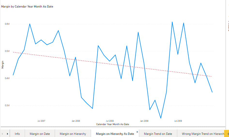
When the X axis contains a hierarchy, and the the Date level is selected, it’s possible to activate the Trend line from the Analytics panel. But changing the level in the line chart to Year Month, the trend line disappears, and a new “i” icon appears with a tooltip stating that there are “Not a Number” values.

A possible solution is to create a Date Hierarchy where every level is of numeric type and the values are contiguous without “jumps”. For instance, representing the Year Month as YYYYMM, like 200801, 200802 would not work, since after 200812 comes 200901, missing all the values between 200813 and 200899.
An awesome solution is proposed by the SQLBI article Creating a simpler and chart-friendly Date table in Power BI. The idea is to represent each level with a date and then to format the date according to the level. This way, the Year Month value is the date of the end of the month, formatted as “mmmm yyyy”, The Year is the date of the end of the year, formatted as “yyyy” and the Year Quarter is the date of the end of the quarter, formatted as … wait there is no format specifier for the quarter!
This is the graph at the Year Month level
This is the same graph at the Year Quarter level. The format is the same as for the Year Month: “mmmm yyyy”

This might be acceptable, but when a better format for the axis is required, it’s possible to write a “Trend” measure to be used instead of the Analytics Trend line.
The DAX formuia for the “Trend” measure is a straightforward implementation of the Simple Linear Regression, but care must be taken when used with a Date Hierarchy, since it is not additive and the formula has to be implemented for each level of the hierarchy. I “took inspiration” from Daniil Maslyuk’s blog post Simple linear regression in DAX, and I implemented the formula from wikipedia.
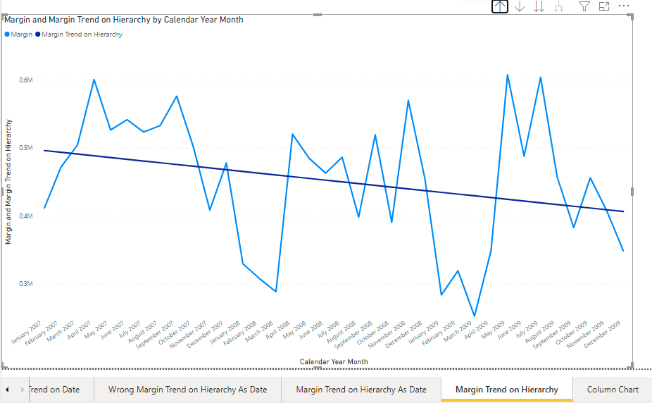
This is the resulting line chart with the non-numeric Date Hierarchy at the Year Month level
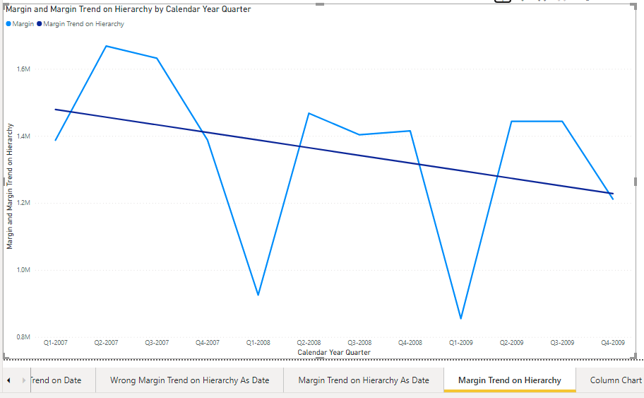
And at the Year Quarter level
Using the same technique it’s possible to implement other “Trend” measures, for instance a “Total trend” measure to implement a Trend line unaffected by slicers.
Another advantage is that trend measures can be used with visuals that don’t have the Analytics panel.
“Trend” measure DAX code must be replicated per each measure that requires a tend line, and therefore it can be tedious. The usual approach not to replicate DAX code is by using calculation groups. I’m planning to give it a try in the near future.
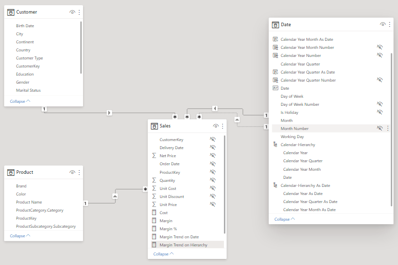
The model
The sample model is built starting from the ContosRetailDW DB that comes with “The Definitive Guide to DAX – Second edition” book companion and is a star schema of the Sales, Customer, Product and Date tables.
The measures are very simple
Cost = SUMX(Sales, Sales[Quantity] * Sales[Unit Cost])
Sales Amount = SUMX(Sales, Sales[Quantity] * Sales[Net Price])
Margin = [Sales Amount] - [Cost]
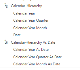
Margin % = DIVIDE( [Margin], [Sales Amount] )The following calculated columns are needed to build the “Calendar-Hierarchy as Date”, required to implement the solution from the SQLBI article
Calendar Year As Date = ENDOFYEAR( 'Date'[Date] )

Calendar Year Quarter As Date = ENDOFQUARTER( 'Date'[Date] )

Calendar Year Month As Date = ENDOFMONTH( 'Date'[Date] )
The contiguous numeric calculated columns are used for the “Trend” measure
Calendar Year Number = YEAR( 'Date'[Date] ) - YEAR( MIN( 'Date'[Date] ) )

Calendar Year Quarter Number = 'Date'[Calendar Year Number] * 4
    + QUARTER ( 'Date'[Date] ) - 1

Calendar Year Month Number = 'Date'[Calendar Year Number] * 12
    + MONTH( 'Date'[Date] ) - 1
The two “Calendar-Hierarchy” are
The “Trend” measure code
The first version of the “Trend” measure for the [Margin] is the [Margin Trend on Date], that can be used when ‘Date'[Date] is selected for the X axis
Margin Trend on Date =
IF (
    NOT ISBLANK ( [Margin] ),
    VAR Tab =
        FILTER (
            CALCULATETABLE (
                SELECTCOLUMNS (
                    'Date',
                    "@X", CONVERT ( 'Date'[Date], DOUBLE ),
                    "@Y", CONVERT ( [Margin], DOUBLE )
                ),
                ALLSELECTED ( 'Date' )
            ),
            NOT ISBLANK ( [@X] ) && NOT ISBLANK ( [@Y] )
        )
    VAR SX =
        SUMX ( Tab, [@X] )
    VAR SY =
        SUMX ( Tab, [@Y] )
    VAR SX2 =
        SUMX ( Tab, [@X] * [@X] )
    VAR SXY =
        SUMX ( Tab, [@X] * [@Y] )
    VAR N =
        COUNTROWS ( Tab )
    VAR Denominator = N * SX2 - SX * SX
    VAR Slope =
        DIVIDE ( N * SXY - SX * SY, Denominator )
    VAR Intercept =
        DIVIDE ( SY * SX2 - SX * SXY, Denominator )
    VAR V =
        Intercept
            + Slope * VALUES ( 'Date'[Date] )
    RETURN
        V
)
The IF condition is needed to avoid the calculation when the measure for the current date is BLANK().
Then the Tab table variable is declared, to contain all the pairs of Date and Margin values in the filter context of the visual. This is obtained by means of ALLSELECTED( ‘Date’ ) inside CALCULATETABLE(). The conversion to DOUBLE in this sample is needed to avoid an arithmetic overflow caused by multiplications. The remaining code is the straightforward implementation of the Simple Linear Regression formula, to compute the Y for the current ‘Date'[Date].
This graph shows the Margin Trend on Date measure perfectly overlapping the Trend line.

But this formula only works when ‘Date'[Date] is set as the X axis. This because the bit of code that computes the V variable makes use of VALUES( ‘Date'[Date] ), that is converted to a scalar value when it contains a single row, but it returns error when it contains more than one row.
VAR V = Intercept + Slope * VALUES ( 'Date'[Date] )The first idea that comes to mind is to add an aggregator: [Margin] is additive, therefore is [Margin Trend] also additive? The answer is no, because of mathematics.
The following is an attempt (failed attempt) to implement an aggregation that, as expected, does not work
Wrong Margin Trend on Hierarchy =
IF (
    NOT ISBLANK ( [Margin] ),
    VAR Tab =
        FILTER (
            CALCULATETABLE (
                SELECTCOLUMNS (
                    'Date',
                    "@X", CONVERT ( 'Date'[Date], DOUBLE ),
                    "@Y", CONVERT ( [Margin], DOUBLE )
                ),
                ALLSELECTED ( 'Date' )
            ),
            NOT ISBLANK ( [@X] ) && NOT ISBLANK ( [@Y] )
        )
    VAR SX =
        SUMX ( Tab, [@X] )
    VAR SY =
        SUMX ( Tab, [@Y] )
    VAR SX2 =
        SUMX ( Tab, [@X] * [@X] )
    VAR SXY =
        SUMX ( Tab, [@X] * [@Y] )
    VAR N =
        COUNTROWS ( Tab )
    VAR Denominator = N * SX2 - SX * SX
    VAR Slope =
        DIVIDE ( N * SXY - SX * SY, Denominator )
    VAR Intercept =
        DIVIDE ( SY * SX2 - SX * SXY, Denominator )
    VAR V =
        SUMX ( DISTINCT ( 'Date'[Date] ), Intercept + Slope * 'Date'[Date] )
    RETURN
        V
)
And this is the graph showing that the [Wrong Margin Trend on Hierarchy] is not a straight line and even that its own Trend line (purple dotted) doesn’t match with the [Margin] Trend Line (blue dotted)

The correct solution is to test the current hierarchy level with ISINSCOPE and implement the formula accordingly. Which is very long and tedious
Margin Trend on Hierarchy =
IF (
    NOT ISBLANK ( [Margin] ),
    SWITCH (
        TRUE,
        ISINSCOPE ( 'Date'[Date] ),
            VAR Tab =
                FILTER (
                    CALCULATETABLE (
                        SELECTCOLUMNS (
                            'Date',
                            "@X", CONVERT ( 'Date'[Date], DOUBLE ),
                            "@Y", CONVERT ( [Margin], DOUBLE )
                        ),
                        ALLSELECTED ( 'Date' )
                    ),
                    NOT ISBLANK ( [@X] ) && NOT ISBLANK ( [@Y] )
                )
            VAR SX =
                SUMX ( Tab, [@X] )
            VAR SY =
                SUMX ( Tab, [@Y] )
            VAR SX2 =
                SUMX ( Tab, [@X] * [@X] )
            VAR SXY =
                SUMX ( Tab, [@X] * [@Y] )
            VAR N =
                COUNTROWS ( Tab )
            VAR Denominator = N * SX2 - SX * SX
            VAR Slope =
                DIVIDE ( N * SXY - SX * SY, Denominator )
            VAR Intercept =
                DIVIDE ( SY * SX2 - SX * SXY, Denominator )
            VAR V =
                Intercept
                    + Slope * VALUES ( 'Date'[Date] )
            RETURN
                V,
        ISINSCOPE ( 'Date'[Calendar Year Month] )
            || ISINSCOPE ( 'Date'[Calendar Year Month Number] )
            || ISINSCOPE ( 'Date'[Calendar Year Month As Date] ),
            VAR Tab =
                FILTER (
                    CALCULATETABLE (
                        SELECTCOLUMNS (
                            SUMMARIZE ( 'Date', 'Date'[Calendar Year Month Number] ),
                            "@X", CONVERT ( 'Date'[Calendar Year Month Number], DOUBLE ),
                            "@Y", CONVERT ( [Margin], DOUBLE )
                        ),
                        ALLSELECTED ( 'Date' )
                    ),
                    NOT ISBLANK ( [@X] ) && NOT ISBLANK ( [@Y] )
                )
            VAR SX =
                SUMX ( Tab, [@X] )
            VAR SY =
                SUMX ( Tab, [@Y] )
            VAR SX2 =
                SUMX ( Tab, [@X] * [@X] )
            VAR SXY =
                SUMX ( Tab, [@X] * [@Y] )
            VAR N =
                COUNTROWS ( Tab )
            VAR Denominator = N * SX2 - SX * SX
            VAR Slope =
                DIVIDE ( N * SXY - SX * SY, Denominator )
            VAR Intercept =
                DIVIDE ( SY * SX2 - SX * SXY, Denominator )
            VAR V =
                Intercept
                    + Slope * VALUES ( 'Date'[Calendar Year Month Number] )
            RETURN
                V,
        ISINSCOPE ( 'Date'[Calendar Year Quarter] )
            || ISINSCOPE ( 'Date'[Calendar Year Quarter Number] )
            || ISINSCOPE ( 'Date'[Calendar Year Quarter As Date] ),
            VAR Tab =
                FILTER (
                    CALCULATETABLE (
                        SELECTCOLUMNS (
                            SUMMARIZE ( 'Date', 'Date'[Calendar Year Quarter Number] ),
                            "@X", CONVERT('Date'[Calendar Year Quarter Number], DOUBLE),
                            "@Y", CONVERT([Margin], DOUBLE)
                        ),
                        ALLSELECTED ( 'Date' )
                    ),
                    NOT ISBLANK ( [@X] ) && NOT ISBLANK ( [@Y] )
                )
            VAR SX =
                SUMX ( Tab, [@X] )
            VAR SY =
                SUMX ( Tab, [@Y] )
            VAR SX2 =
                SUMX ( Tab, [@X] * [@X] )
            VAR SXY =
                SUMX ( Tab, [@X] * [@Y] )
            VAR N =
                COUNTROWS ( Tab )
            VAR Denominator = N * SX2 - SX * SX
            VAR Slope =
                DIVIDE ( N * SXY - SX * SY, Denominator )
            VAR Intercept =
                DIVIDE ( SY * SX2 - SX * SXY, Denominator )
            VAR V =
                Intercept
                    + Slope * VALUES ( 'Date'[Calendar Year Quarter Number] )
            RETURN
                V,
        ISINSCOPE ( 'Date'[Calendar Year] )
            || ISINSCOPE ( 'Date'[Calendar Year Number] )
            || ISINSCOPE ( 'Date'[Calendar Year As Date] ),
            VAR Tab =
                FILTER (
                    CALCULATETABLE (
                        SELECTCOLUMNS (
                            SUMMARIZE ( 'Date', 'Date'[Calendar Year Number] ),
                            "@X", CONVERT('Date'[Calendar Year Number], DOUBLE),
                            "@Y", CONVERT([Margin], DOUBLE)
                        ),
                        ALLSELECTED ( 'Date' )
                    ),
                    NOT ISBLANK ( [@X] ) && NOT ISBLANK ( [@Y] )
                )
            VAR SX =
                SUMX ( Tab, [@X] )
            VAR SY =
                SUMX ( Tab, [@Y] )
            VAR SX2 =
                SUMX ( Tab, [@X] * [@X] )
            VAR SXY =
                SUMX ( Tab, [@X] * [@Y] )
            VAR N =
                COUNTROWS ( Tab )
            VAR Denominator = N * SX2 - SX * SX
            VAR Slope =
                DIVIDE ( N * SXY - SX * SY, Denominator )
            VAR Intercept =
                DIVIDE ( SY * SX2 - SX * SXY, Denominator )
            VAR V =
                Intercept
                    + Slope * VALUES ( 'Date'[Calendar Year Number] )
            RETURN
                V
    )
)
The ISINSCOPE tests might change according to the existing hierarchies. This sample model has two of them based on different columns.
The [Margin Trend on Hierarchy] can be tested against the Trend line using the Calendar-Hierarchy As Date at the Year Month level

And at the Year Quarter level
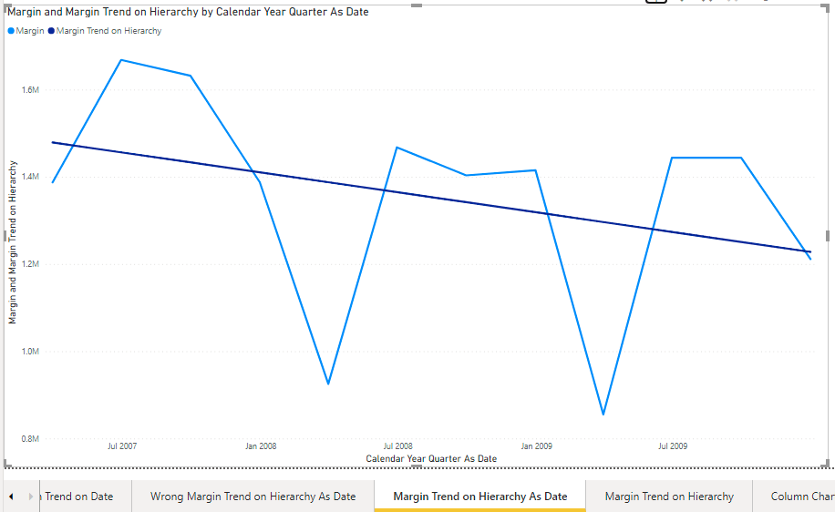
The Trend line and the [Margin Trend on Hierarchy] overlap just as expected.
Finally the [Margin Trend on Hierarchy] measure can be used with the plain Calendar-Hierarchy


The [Margin Trend on Hierarchy] can be used with other kind of visuals and even when the [Margin] measure is not selected. Here we have the Margin trend line over a [Sales Amount] per Year Month column chart.

The sample pbix file can be downloaded from my Github project.
