I've been working on Business Intelligence since 2007, developing ETLs and OLAP cubes with Microsoft SQL Server products suite. My actual main interests are on the DAX language and Power BI.
A few weeks ago I read a question on matrix multiplication with DAX. The user asked if it was possible to implement matrix multiplication using DAX and how.
The answer is that the DAX language doesn’t have the matrix construct, and therefore the best solution is to move the matrix multiplication at the source level using a more suitable language. Even if an implementation was possible, it would be a complex and awkward code, that would be inefficient and hard to read.
The purpose of this article is to show some inefficient and hard-to-read code that does matrix multiplication. It’s meant for DAX and mathematics geeks to have some fun.
The first problem to solve is how to represent matrix with DAX. Using a table directly as a matrix would not be possible, since DAX tables cannot be indexed by row and column indexes
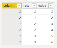
The solution I found is to implement a table with a row per each cell, with row, column and value columns
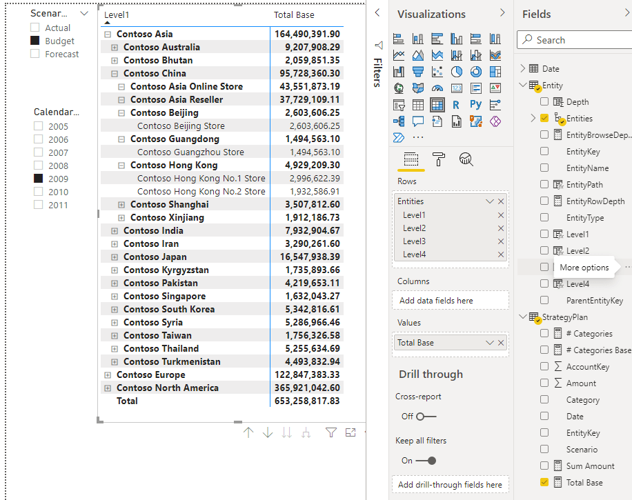
This table representation of a matrix can be shown in a report as a matrix using the Matrix visual, with the column row on the Rows, the column on the Columns, and the value on the Values, which is pretty straightforward.
Having row and column indexes, it becomes possible to implement matrix multiplication. To access the single value of a cell, I used the LOOKUPVALUE DAX function, that in my opinion is the more readable function for that purpose.
This code returns a table. The resulting table will use the same matrix representation using the row, column and value columns.
The multiplication of a matrix with l rows and m columns times a matrix with m rows and n columns will return a matrix with l rows and n columns. The details on how matrix multiplication works can be found on wikipedia Matrix multiplication page .
The code multiplies matrix A with matrix B. Matrixes can be of any size, but to keep code simple there is no test on the condition that the number of columns of A are equal to the number of columns of B.
The GENERATE iterates on the rows of matrix A, and then, per each row it executes the ADDCOLUMNS to iterate on the columns of table B.
Per each pair of values of A[row] and B[colum], the SUMX is executed to iterate on A[column].
In this explanation we will indicate A[row] as r, B[column] as c and A[column] as i, so we can indicate a matrix cell as Matrix(row, column), like for instance A(r, i).
Per each iteration the LOOKUPVALUES are used to retrieve the A(c, i) and B(i, c) elements to be multiplied and then added up by the SUMX.
In conclusion, this code is not so hard-to-read, but it assumes that we have a suitable representation for the matrixes and the result is a table.
More code would be unavoidable to be able to first prepare the matrix representation and implementing the multiplication using a measure instead of a calculated table could be harder. But I still didn’t try it, maybe in the future.
For my sample I implemented two small matrixes using the DATATABLE function
In this post I’m showing how to create random data with Power Query that doesn’t change when a refresh operation happens. In my previous post Loading Large Random Datasets with Power Query I used Number.Random() and Number.RandomBetween(), that generate a different random number each time they are called. The consequence is that each time we refresh the dataset we get a new set of random values, and therefore it is impossible to check the consistency of the results we get by our measures after a modification in Power Query triggers a refresh operation. A solution is to use the List.Random() function, that returns a list of random numbers and has an optional seed parameter. When the same seed is specified, List.Random() returns the same list of random values. But List.Random() returns a list of numbers and therefore cannot directly replace Number.RandomBetween() in the code shown in the previous post: first we have to generate the list with all the random numbers we need and then we must access the list taking the random number at the right index. Last but not least, the Number.RandBetween() generates a number in the specified range and List.Random() instead generates a list of numbers between 0 and 1, so we must also change the code that computes the final value.
The signature of List.Random() is
List.Random(count as number, optional seed as nullable number) as list
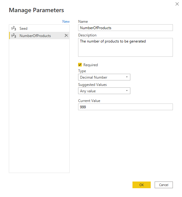
So we must specify the number of random numbers to be generated as the count parameter and the seed to be used. In our example the count is the same value used to generate the list of indexes, that is the length of the Fake Product table. The seed can be any value, its only purpose is to make the generated random numbers list to be the same across refreshes. Changing the seed can be useful to check the resulting model using different values. Since the same length value is to be used in two different places, I created a parameter called NumberOfProducts
I also created a parameter called Seed to be used as the seed Therefore the code to generate the list of random values and the list of indexes becomes
and the code to access the RandomList at the index corresponding to the line becomes
RandomList{[ID] - 1}
the curly braces are used to access the list at the specified index, and the ID between the square brackets refers to the ID column in the current table row. Then, since lists are zero based and the ID index instead is starting at 1, we need to subtract 1 from the ID. After the changes, the final code for the Fake Products table is
Since the number of products is now a parameter, I also had to change the code that computes the name of the product by replacing the format parameter “000” in the Number.ToText() with a string containing a number of zeroes large enough, that is computed as a separated query PadNumber
let
    LogNumber = Number.Log10(NumberOfProducts),
    Digits = Number.RoundUp(LogNumber),
    PadNumber = Text.Repeat("0", Digits)
in
    PadNumber
Building Power BI models for test purpose requires test datasets. Small tables can be inserted directly in Power BI through the Enter Data user interface
When a larger amount of data is needed, we can use external data sources: SQL tables, Excel files, CSV files and so on.
In this article I’m showing a technique to build large random datasets, directly in Power Query, using M language and without the need for any external data source.
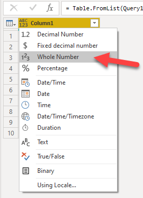
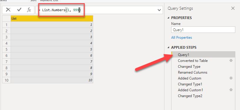
The idea is very simple: starting from the blank query, using the List.Numbers() M function I create a list of integers, then using the Power Query interface “To Table” I transform the list to a table
Since the list just contains numbers, I just accept the defaults and click the OK button
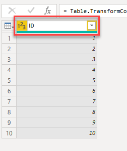
And finally I set the type and the name of the column to Whole Number and ID
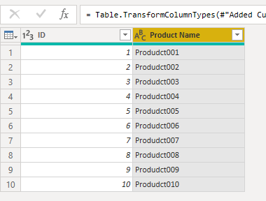
Then I can add new custom columns, for instance the fake name of a product by concatenating “Product” and the ID converted to a string
The Number.ToText() function can take an optional format specifier. In this case I formatted the ID to be a three digit number with leading zeroes.
"Produdct" & Number.ToText([ID], "000")
Last I selected Text for the column type
The final result shows the fake product names
To generate random data we can use the Number.Random() and Number.RandomBetween() functions. Sadly, they don’t accept a seed parameter, therefore using these functions it’s not possible to generate the same dataset twice. When this is an issue, the List.Random() function can be used instead.
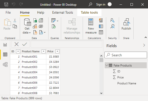
For instance we can generate a Price column with random values in a range from 1 to 5 dollars with two decimals by creating a new custom column like before, but using the following M expression
Number.RandomBetween(100, 500) / 100
And this is the result, after selecting Fixed Decimal Type
After adding all the desired custom columns we can generate as many rows as needed just by changing the Number.List() parameters
And after renaming the query to Fake Products
I can finally close Power Query Editor to load the data into the Power BI dataset
A larger dataset
Using this technique, I was able to change the large model from my previous article Loading 1.6 Billion Rows Snapshot Table with Power Query to work without the need of the source DB. Also, since I can change the size of the dataset at will, I can now share it with a small dataset, that can be made great as you please after the download.
As a starting point I used the template file from my former article HeadCount snapshot M – big.pbit, then I changed the M code in the Employees query using the technique show before.
I also added a few parameters to better control the dataset generation
EmployeeMaxNumber [Number]: the total number of fake employees to be generated
FirstDate [Date]: the lower bound for the hire and leave dates
LastDate [Date]: the upper bound for the hire and leave dates
MinimumDays [Number]: the minimum days of stay
LeaveProbability [Number]: the probability that the employee left (from 0 to 1)
The M code to generate a random date requires the conversions from Date to Number and vice-versa
Since I changed the date range I also had to apply a few minor changes to M code for the Employee Snapshot table and to the DAX code for the Date table.
Setting EmployeeMaxNumber to one million, I generated a snapshot table around 1.7 billion rows. This number can vary, since it’s a function of the random generated dates.
Conclusions
Power Query can be used to generate test datasets as large as needed thanks to the List.Numbers(), Number.Random() and Number.RandomBetween() M functions.
When I implemented the C# script for my last post I had to replicate some code, since advanced scripting in Tabular Editor as is doesn’t provide a way to define functions.
But starting from C# version 7.0 it’s possible to declare local functions, and both Tabular Editor versions, the free and the commercial ones, allow to specify the C# compiler to be used and the language version.
Therefore I decided to see if local functions could be used with advanced scripting.
They do, and I was able to remove the duplicate code from my last C# script.
I configured the Roslyn compiler for Tabular Editor 2, the free version
And I also configured it for Tabular Editor 3, the commercial version
The Roslyn compiler path on my PC is C:\Program Files (x86)\Microsoft Visual Studio\2019\Enterprise\MSBuild\Current\Bin\Roslyn
It might be different on other installations
The language version I specified is the 8.0, using the corresponding command line switch for the compiler -langversion:8.0
With this version of the compiler we can use local functions that are private methods defined inside another method and can be called only from the method that contains it. This allows us to declare functions, since the script we write is wrapped by Tabular Editor inside a method.
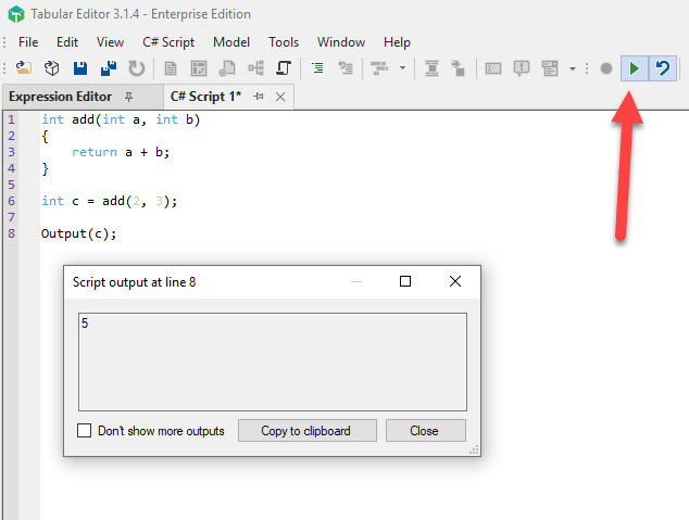
For instance, opening a new script we can implement a function that adds two numbers and calls it (here I’m using TE3, but it also works in TE2)
We write the simple script that follows and we run it using the Run Script button
int add(int a, int b)
{
    return a + b;
}

int c = add(2, 3);

Output(c);
The Output() method shows its argument inside a popup window
And that’s it, once I verified that the local functions worked, I changed the C# script that generates the Parent-Child hierarchy of my last post adding the “local functions” section and replacing the duplicate code using functions instead.
// configuration start

int levels = 4;
int previouslevels = 4;

string tableName = "Entity";
string pathName = "EntityPath";
string keyName = "EntityKey";
string nameName = "EntityName";
string parentKeyName = "ParentEntityKey";
string levelNameFormat = "Level{0}";
string depthName = "Depth";
string rowDepthMeasureName = "EntityRowDepth";
string browseDepthMeasureName = "EntityBrowseDepth";
string wrapperMeasuresTableName = "StrategyPlan";
string hierarchyName = "Entities";
var wrapperMeasuresTable = Model.Tables[wrapperMeasuresTableName];
SortedDictionary<string, string> measuresToWrap =
    new SortedDictionary<string, string>
{
    { "# Categories", "# Categories Base"},
    { "Sum Amount", "Total Base" }
};
// configuration end

// local functions

void DeleteHierarchy(string hierarchyName, string tableName)
{
    var table = Model.Tables[tableName];
    var hierarchiesCollection = table.Hierarchies.Where(
        m => m.Name == hierarchyName );
    if (hierarchiesCollection.Count() > 0)
    {
        hierarchiesCollection.First().Delete();
    }
}

void DeleteMeasure(string measureName, string tableName)
{
    var table = Model.Tables[tableName];
    var measuresCollection = table.Measures.Where(
        m => m.Name == measureName );
    if (measuresCollection.Count() > 0)
    {
        measuresCollection.First().Delete();
    }
}


void DeleteCalculatedColumn(string calculatedColumnName, string tableName)
{
    var table = Model.Tables[tableName];
    var calculatedColumnsCollection = table.CalculatedColumns.Where(
        m => m.Name == calculatedColumnName );
    if (calculatedColumnsCollection.Count() > 0)
    {
        calculatedColumnsCollection.First().Delete();
    }
}

// cleanup
DeleteHierarchy(hierarchyName, tableName);
foreach (var wrapperMeasurePair in measuresToWrap)
{
    DeleteMeasure(wrapperMeasurePair.Value, wrapperMeasuresTableName);
}
DeleteMeasure(browseDepthMeasureName, tableName);
DeleteMeasure(rowDepthMeasureName, tableName);
DeleteCalculatedColumn(depthName, tableName);
for (int i = 1; i <= previouslevels; ++i)
{
    string levelName = string.Format(levelNameFormat, i);
    DeleteCalculatedColumn(levelName, tableName);
}
DeleteCalculatedColumn(pathName, tableName);

// create calculated columns
string daxLevelFormat =
@"VAR LevelNumber = {0}
VAR LevelKey = PATHITEM( {1}[{2}], LevelNumber, INTEGER )
VAR LevelName = LOOKUPVALUE( {1}[{3}], {1}[{4}], LevelKey )
VAR Result = LevelName
RETURN
    Result
";

string daxPath = string.Format( "PATH({0}[{1}], {0}[{2}])",
    tableName, keyName, parentKeyName);
var table = Model.Tables[tableName];
table.AddCalculatedColumn(pathName, daxPath);

for (int i = 1; i <= levels; ++i)
{
    string levelName = string.Format(levelNameFormat, i);
    string daxLevel = string.Format(daxLevelFormat, i,
        tableName, pathName, nameName, keyName);
    table.AddCalculatedColumn(levelName, daxLevel);
}

string daxDepthFormat = "PATHLENGTH( {0}[{1}] )";
string daxDepth = string.Format(
    daxDepthFormat, tableName, pathName);
table.AddCalculatedColumn(depthName, daxDepth);


// Create Hierarchy

table.AddHierarchy(hierarchyName);
for (int i = 1; i <= levels; ++i)
{
    string levelName = string.Format(levelNameFormat, i);
    string daxLevel = string.Format(daxLevelFormat, i,
        tableName, pathName, nameName, keyName);
    table.Hierarchies[hierarchyName].AddLevel(levelName);
}

// Create measures
string daxRowDepthMeasureFormat = "MAX( {0}[{1}])";
string daxRowDepthMeasure = string.Format(
    daxRowDepthMeasureFormat, tableName, depthName );
table.AddMeasure(rowDepthMeasureName, daxRowDepthMeasure);

string daxBrowseDepthMeasure = "";
for (int i = 1; i <= levels; ++i)
{
    string levelMeasureFormat = "ISINSCOPE( {0}[{1}] )";
    string levelName = string.Format(levelNameFormat, i);
    daxBrowseDepthMeasure += string.Format(
        levelMeasureFormat, tableName, levelName);
    if (i < levels)
    {
        daxBrowseDepthMeasure += " + ";
    }
}
table.AddMeasure(browseDepthMeasureName, daxBrowseDepthMeasure);

string daxWrapperMeasureFormat =
@"VAR Val = [{0}]
VAR ShowRow = [{1}] <= [{2}]
VAR Result = IF( ShowRow, Val )
RETURN
    Result
";

foreach (var wrapperMeasurePair in measuresToWrap)
{
    string daxWrapperMeasure = string.Format(daxWrapperMeasureFormat,
        wrapperMeasurePair.Key, // measure to be wrapped
        browseDepthMeasureName,
        rowDepthMeasureName);
    wrapperMeasuresTable.AddMeasure(wrapperMeasurePair.Value, daxWrapperMeasure);

}

table.Measures.FormatDax(false);
wrapperMeasuresTable.Measures.FormatDax(false);
Implementing Parent-Child hierarchies in DAX requires the usage of a special set of functions, PATH, PATHITEM and PATHLENGTH, specifically designed for this purpose. These functions are used to flatten the hierarchy as as set of calculated columns. This means that the depth of the hierarchy is fixed and limited to the number of calculated columns that was decided at design time.
When the depth increases, new calculated columns must be added. This, together with the fact that I quickly forget how to use the PATH* functions, since I use them only when dealing with parent-child hierarchies, gave me the idea to write a script to automatically generate parent-child hierarchies.
As a test project I decided to implement a script to re-create the basic parent-child DAX pattern described in the Parent-child hierarchies DAX pattern
My conclusion is that this kind of script can be written and works smoothly, but it requires to enable the unsupported features of Power BI in settings of Tabular Editor.
Since I wrote the script using variables to contain the names in the model, it should be easily adapted to other models too, but I still have to try it.
This is the report built using the script generated parent-child hierarchy
Loading and Executing The Script
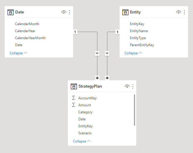
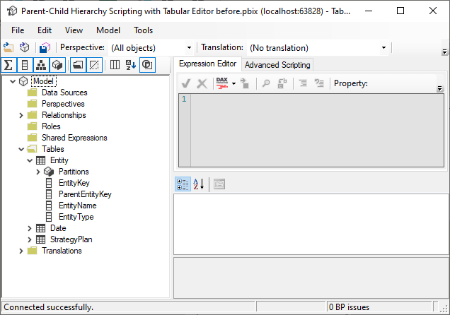
As a start point I used a small model containing only three tables, that I saved as the “Parent-Child Hierarchy Scripting with Tabular Editor before.pbix” file.
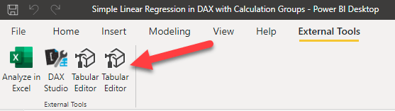
Then to ran Tabular Editor 2 we click on its icon from the External Tools ribbon of Power BI
In Tabular Editor we can see the Entity table only has four columns
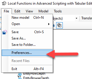
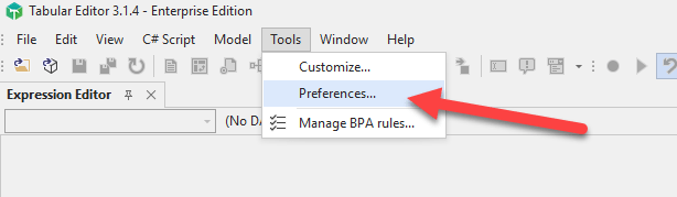
Then we have to enable the Unsupported Power BI features in the Preferences (through the File->Preferences… menu)
This is necessary, otherwise an attempt to create a calculated column generates the following error
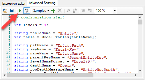
The Advanced Scripting tab shows the editor where the script can be written, and the “load”, “save” and “run” buttons
By clicking on the “Load” button and selecting the “Parent-Child Hierarchy.cs” file the script appears in the edit window and can be executed
The result is that the calculated columns and the measures of the pattern are generated. Finally we must click on the button to save the changes to the connected Power BI model.
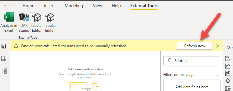
After saving the model to Power BI, we must click on the “Refresh Now” button to answer the Power BI request to manually refresh the model
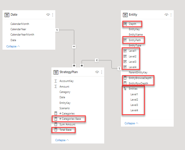
Finally we can find the generated calculated columns, measures and hierarchy in the model
The first part of the script contains a configuration section with a list of variables that can be used to adapt the script to other models. The first one is the “levels” variables, that contains the number of “level” columns to be generated, that corresponds to the maximum depth allowed for the hierarchy.
Here follows the entire script, that just follows the pattern description step by step, with the only difference that I added an additional measure [# categories base], that is just for testing purpose.
// configuration start

int levels = 4;

string tableName = "Entity";
var table = Model.Tables[tableName];

string pathName = "EntityPath";
string keyName = "EntityKey";
string nameName = "EntityName";
string parentKeyName = "ParentEntityKey";
string levelNameFormat = "Level{0}";
string depthName = "Depth";
string rowDepthMeasureName = "EntityRowDepth";
string browseDepthMeasureName = "EntityBrowseDepth";
string wrapperMeasuresTableName = "StrategyPlan";
string hierarchyName = "Entities";
var wrapperMeasuresTable = Model.Tables[wrapperMeasuresTableName];
SortedDictionary<string, string> measuresToWrap =
    new SortedDictionary<string, string>
{
    { "# Categories", "# Categories Base"},
    { "Sum Amount", "Total Base" }
};
// configuration end

string daxPath = string.Format( "PATH({0}[{1}], {0}[{2}])",
    tableName, keyName, parentKeyName);


// cleanup

var hierarchiesCollection = table.Hierarchies.Where(
    m => m.Name == hierarchyName );
if (hierarchiesCollection.Count() > 0)
{
    hierarchiesCollection.First().Delete();
}


foreach (var wrapperMeasurePair in measuresToWrap)
{
    var wrapperMeasuresCollection = wrapperMeasuresTable.Measures.Where(
        m => m.Name == wrapperMeasurePair.Value );
    if (wrapperMeasuresCollection.Count() > 0)
    {
        wrapperMeasuresCollection.First().Delete();
    }
}

var browseDepthMeasureCollection = table.Measures.Where(
    m => m.Name == browseDepthMeasureName );
if (browseDepthMeasureCollection.Count() > 0)
{
    browseDepthMeasureCollection.First().Delete();
}

var rowDepthMeasureCollection = table.Measures.Where(
    m => m.Name == rowDepthMeasureName );
if (rowDepthMeasureCollection.Count() > 0)
{
    rowDepthMeasureCollection.First().Delete();
}

var depthCollection = table.CalculatedColumns.Where(
    m => m.Name == depthName );
if (depthCollection.Count() > 0)
{
    depthCollection.First().Delete();
}

for (int i = 1; i <= levels; ++i)
{
    string levelName = string.Format(levelNameFormat, i);
    var levelCalculatedColumnCollection =
        table.CalculatedColumns.Where( m => m.Name == levelName );
    if (levelCalculatedColumnCollection.Count() > 0)
    {
        levelCalculatedColumnCollection.First().Delete();
    }
}

var pathCalculatedColumnCollection = table.CalculatedColumns.Where(
    m => m.Name == pathName );
if (pathCalculatedColumnCollection.Count() > 0)
{
    pathCalculatedColumnCollection.First().Delete();
}

// create calculated columns
table.AddCalculatedColumn(pathName, daxPath);

string daxLevelFormat =
@"VAR LevelNumber = {0}
VAR LevelKey = PATHITEM( {1}[{2}], LevelNumber, INTEGER )
VAR LevelName = LOOKUPVALUE( {1}[{3}], {1}[{4}], LevelKey )
VAR Result = LevelName
RETURN
    Result
";

for (int i = 1; i <= levels; ++i)
{
    string levelName = string.Format(levelNameFormat, i);
    string daxLevel = string.Format(daxLevelFormat, i,
        tableName, pathName, nameName, keyName);
    table.AddCalculatedColumn(levelName, daxLevel);
}

string daxDepthFormat = "PATHLENGTH( {0}[{1}] )";
string daxDepth = string.Format(
    daxDepthFormat, tableName, pathName);
table.AddCalculatedColumn(depthName, daxDepth);


// Create Hierarchy

table.AddHierarchy(hierarchyName);
for (int i = 1; i <= levels; ++i)
{
    string levelName = string.Format(levelNameFormat, i);
    string daxLevel = string.Format(daxLevelFormat, i,
        tableName, pathName, nameName, keyName);
    table.Hierarchies[hierarchyName].AddLevel(levelName);
}

// Create measures
string daxRowDepthMeasureFormat = "MAX( {0}[{1}])";
string daxRowDepthMeasure = string.Format(
    daxRowDepthMeasureFormat, tableName, depthName );
table.AddMeasure(rowDepthMeasureName, daxRowDepthMeasure);

string daxBrowseDepthMeasure = "";
for (int i = 1; i <= levels; ++i)
{
    string levelMeasureFormat = "ISINSCOPE( {0}[{1}] )";
    string levelName = string.Format(levelNameFormat, i);
    daxBrowseDepthMeasure += string.Format(
        levelMeasureFormat, tableName, levelName);
    if (i < levels)
    {
        daxBrowseDepthMeasure += " + ";
    }
}
table.AddMeasure(browseDepthMeasureName, daxBrowseDepthMeasure);

string daxWrapperMeasureFormat =
@"VAR Val = [{0}]
VAR ShowRow = [{1}] <= [{2}]
VAR Result = IF( ShowRow, Val )
RETURN
    Result
";

foreach (var wrapperMeasurePair in measuresToWrap)
{
    string daxWrapperMeasure = string.Format(daxWrapperMeasureFormat,
        wrapperMeasurePair.Key, // measure to be wrapped
        browseDepthMeasureName,
        rowDepthMeasureName);
    wrapperMeasuresTable.AddMeasure(wrapperMeasurePair.Value, daxWrapperMeasure);

}

table.Measures.FormatDax(false);
wrapperMeasuresTable.Measures.FormatDax(false);
The documentation about the Advanced Scripting can be found on the Tabular Editor site,
In my previous post Simple Linear Regression in DAX with Calculation Groups I used Calculation Groups to avoid code duplication for the Trending Measures. A possible alternative to avoid manually duplicated code, is by writing a program to automatically duplicate code.
Tabular Editor Advanced Scripting panel allows editing and running scripts written in c# to automatically change the model. And the editor also has the intellisense!
Tabular Editor exposes an object interface, through which the script can manipulate the model. Debugging in Tabular Editor can be done with the Output() function, that shows the content of its parameter in a popup window.
Output() can also be used as a method, applied to the object to be shown
The generated DAX Code can also be formatted using the FormatDax() method.
Scripts can also be executed by running Tabular Editor from the command line with the -S parameter. This can become very interesting when trying to build a CI/CD environment.
I wrote a parametrized script to automatically generate the Trending measures for [Sales Amount], [Margin] and [Margin %] using both hierarchies over Year, Quarter, Month and Date of the previous post, the Calendar-Hierarchy and the Calendar-Hierarchy as Date.
The parameters are
The name of the table containing the measures
The name of the table containing the hierarchies.
The list of the levels of the hierarchies, each level consisting of the list of columns for the current level.
The list of measures for which the Trending Measure is to be generated.
string tableForMeasures = "Sales";

// Table to be uses for the Hierarchy
string hierarchyTable = "Date";

// Hierarchy levels from higher to lower granularity
// each level contains the list of the columns to be
// considered for the ISINSCOPE condition
// the first one is used as X value for the calculation
// and must be of numeric type
List<string> level1 = new List<string> { "Date" };
List<string> level2 = new List<string> {
    "Calendar Year Month Number",
    "Calendar Year Month",
    "Calendar Year Month As Date" };
List<string> level3 = new List<string> {
    "Calendar Year Quarter Number",
    "Calendar Year Quarter",
    "Calendar Year Quarter As Date" };
List<string> level4 = new List<string> {
    "Calendar Year Number",
    "Calendar Year",
    "Calendar Year As Date" };

List<List<string>> levels = new List<List<string>> {
    level1, level2, level3, level4};


// the measures for which the Trend measure is to be generated
List<string> measures = new List<string> {
    "Margin", "Margin %", "Sales Amount" };
Running the script, I generated the measures [Sales Amount Trend], [Margin Trend] and [Margin % Trend]
That can be used as usual, like in the previous posts
Conclusions
Scripting for generating DAX code is a powerful tool, to be considered when many similar measures are to be written. The simple interface makes writing scripts easier than expected. In the maintenance phase, scripts will allow quick modification of group of measures to be done in a snap.
The script
As a first step to create the script, we must run Tabular Editor from the Power BI External Tool Ribbon
this opens Tabular Editor, automatically connected to Power BI
Then we must select the Advanced Scripting panel and we can start writing the code.
Margin Trend on Hierarchy =
IF (
    NOT ISBLANK ( [Margin] ),
    SWITCH (
        TRUE,
        ISINSCOPE ( 'Date'[Date] ),
            VAR Tab =
                FILTER (
                    CALCULATETABLE (
                        SELECTCOLUMNS (
                            'Date',
                            "@X", CONVERT ( 'Date'[Date], DOUBLE ),
                            "@Y", CONVERT ( [Margin], DOUBLE )
                        ),
                        ALLSELECTED ( 'Date' )
                    ),
                    NOT ISBLANK ( [@X] ) && NOT ISBLANK ( [@Y] )
                )
            VAR SX =
                SUMX ( Tab, [@X] )
            VAR SY =
                SUMX ( Tab, [@Y] )
            VAR SX2 =
                SUMX ( Tab, [@X] * [@X] )
            VAR SXY =
                SUMX ( Tab, [@X] * [@Y] )
            VAR N =
                COUNTROWS ( Tab )
            VAR Denominator = N * SX2 - SX * SX
            VAR Slope =
                DIVIDE ( N * SXY - SX * SY, Denominator )
            VAR Intercept =
                DIVIDE ( SY * SX2 - SX * SXY, Denominator )
            VAR V =
                Intercept
                    + Slope * VALUES ( 'Date'[Date] )
            RETURN
                V,
        ISINSCOPE ( 'Date'[Calendar Year Month] )
            || ISINSCOPE ( 'Date'[Calendar Year Month Number] )
            || ISINSCOPE ( 'Date'[Calendar Year Month As Date] ),
            VAR Tab =
                FILTER (
                    CALCULATETABLE (
                        SELECTCOLUMNS (
                            SUMMARIZE ( 'Date', 'Date'[Calendar Year Month Number] ),
                            "@X", CONVERT ( 'Date'[Calendar Year Month Number], DOUBLE ),
                            "@Y", CONVERT ( [Margin], DOUBLE )
                        ),
                        ALLSELECTED ( 'Date' )
                    ),
                    NOT ISBLANK ( [@X] ) && NOT ISBLANK ( [@Y] )
                )
            VAR SX =
                SUMX ( Tab, [@X] )
            VAR SY =
                SUMX ( Tab, [@Y] )
            VAR SX2 =
                SUMX ( Tab, [@X] * [@X] )
            VAR SXY =
                SUMX ( Tab, [@X] * [@Y] )
            VAR N =
                COUNTROWS ( Tab )
            VAR Denominator = N * SX2 - SX * SX
            VAR Slope =
                DIVIDE ( N * SXY - SX * SY, Denominator )
            VAR Intercept =
                DIVIDE ( SY * SX2 - SX * SXY, Denominator )
            VAR V =
                Intercept
                    + Slope * VALUES ( 'Date'[Calendar Year Month Number] )
            RETURN
                V,
        ISINSCOPE ( 'Date'[Calendar Year Quarter] )
            || ISINSCOPE ( 'Date'[Calendar Year Quarter Number] )
            || ISINSCOPE ( 'Date'[Calendar Year Quarter As Date] ),
            VAR Tab =
                FILTER (
                    CALCULATETABLE (
                        SELECTCOLUMNS (
                            SUMMARIZE ( 'Date', 'Date'[Calendar Year Quarter Number] ),
                            "@X", CONVERT('Date'[Calendar Year Quarter Number], DOUBLE),
                            "@Y", CONVERT([Margin], DOUBLE)
                        ),
                        ALLSELECTED ( 'Date' )
                    ),
                    NOT ISBLANK ( [@X] ) && NOT ISBLANK ( [@Y] )
                )
            VAR SX =
                SUMX ( Tab, [@X] )
            VAR SY =
                SUMX ( Tab, [@Y] )
            VAR SX2 =
                SUMX ( Tab, [@X] * [@X] )
            VAR SXY =
                SUMX ( Tab, [@X] * [@Y] )
            VAR N =
                COUNTROWS ( Tab )
            VAR Denominator = N * SX2 - SX * SX
            VAR Slope =
                DIVIDE ( N * SXY - SX * SY, Denominator )
            VAR Intercept =
                DIVIDE ( SY * SX2 - SX * SXY, Denominator )
            VAR V =
                Intercept
                    + Slope * VALUES ( 'Date'[Calendar Year Quarter Number] )
            RETURN
                V,
        ISINSCOPE ( 'Date'[Calendar Year] )
            || ISINSCOPE ( 'Date'[Calendar Year Number] )
            || ISINSCOPE ( 'Date'[Calendar Year As Date] ),
            VAR Tab =
                FILTER (
                    CALCULATETABLE (
                        SELECTCOLUMNS (
                            SUMMARIZE ( 'Date', 'Date'[Calendar Year Number] ),
                            "@X", CONVERT('Date'[Calendar Year Number], DOUBLE),
                            "@Y", CONVERT([Margin], DOUBLE)
                        ),
                        ALLSELECTED ( 'Date' )
                    ),
                    NOT ISBLANK ( [@X] ) && NOT ISBLANK ( [@Y] )
                )
            VAR SX =
                SUMX ( Tab, [@X] )
            VAR SY =
                SUMX ( Tab, [@Y] )
            VAR SX2 =
                SUMX ( Tab, [@X] * [@X] )
            VAR SXY =
                SUMX ( Tab, [@X] * [@Y] )
            VAR N =
                COUNTROWS ( Tab )
            VAR Denominator = N * SX2 - SX * SX
            VAR Slope =
                DIVIDE ( N * SXY - SX * SY, Denominator )
            VAR Intercept =
                DIVIDE ( SY * SX2 - SX * SXY, Denominator )
            VAR V =
                Intercept
                    + Slope * VALUES ( 'Date'[Calendar Year Number] )
            RETURN
                V
    )
)
The Trending measure consists of a template that repeats itself several times, with little changes for each level of the hierarchy. Therefore it’s possible to leverage the similarities to shorten the code to be written, and also to parametrize the number of levels of the hierarchy for which the measures must be generated.
The first bit is the initial IF with the SWITCH, that contains that “lasagna” of code corresponding to the different levels of the hierarchy.
IF (
    NOT ISBLANK ( [Margin] ),
    SWITCH (
        TRUE,
... lasagna ...
    )
)
Then, the “lasagna” consists of a repetition of the code in the form of
ISINSCOPE ( 'Date'[Calendar Year Quarter] )
    || ISINSCOPE ( 'Date'[Calendar Year Quarter Number] )
    || ISINSCOPE ( 'Date'[Calendar Year Quarter As Date] ),
    VAR Tab =
        FILTER (
            CALCULATETABLE (
                SELECTCOLUMNS (
                    SUMMARIZE ( 'Date',
                                'Date'[Calendar Year Quarter Number] ),
                    "@X", CONVERT('Date'[Calendar Year Quarter Number],
                                   DOUBLE),
                    "@Y", CONVERT([Margin], DOUBLE)
                ),
                ALLSELECTED ( 'Date' )
            ),
            NOT ISBLANK ( [@X] ) && NOT ISBLANK ( [@Y] )
        )
    VAR SX =
        SUMX ( Tab, [@X] )
    VAR SY =
        SUMX ( Tab, [@Y] )
    VAR SX2 =
        SUMX ( Tab, [@X] * [@X] )
    VAR SXY =
        SUMX ( Tab, [@X] * [@Y] )
    VAR N =
        COUNTROWS ( Tab )
    VAR Denominator = N * SX2 - SX * SX
    VAR Slope =
        DIVIDE ( N * SXY - SX * SY, Denominator )
    VAR Intercept =
        DIVIDE ( SY * SX2 - SX * SXY, Denominator )
    VAR V =
        Intercept
            + Slope * VALUES ( 'Date'[Calendar Year Quarter Number] )
    RETURN
        V,
In the first part there is the condition to be checked to select this layer of “lasagna”. This condition must become a parameter be generated by calling ISINSCOPE() on the corresponding columns in the hierarchies. In the code that calculates the Simple Linear Regression the parameters are
‘Date’: The table
‘Date'[Calendar Year Quarter Number]: the numeric column to be used for the X axis
[Margin]: The measure
So we can transform this snippet of code to the corresponding template, where the placeholderrs for the parametes are reprensented by integer numbers wrapped into curly braces, ready to be used as the format string for the string.Format() method of c#.
string trendMeasureHierarchyLevelFormat = @"
{0},
    VAR Tab =
        FILTER (
            CALCULATETABLE (
                SELECTCOLUMNS (
                    SUMMARIZE ( {1}, {2} ),
                    ""@X"", CONVERT ( {2}, DOUBLE ),
                    ""@Y"", CONVERT ( {3}, DOUBLE )
                ),
                ALLSELECTED ( {1} )
            ),
            NOT ISBLANK ( [@X] ) && NOT ISBLANK ( [@Y] )
        )
    VAR SX =
        SUMX ( Tab, [@X] )
    VAR SY =
        SUMX ( Tab, [@Y] )
    VAR SX2 =
        SUMX ( Tab, [@X] * [@X] )
    VAR SXY =
        SUMX ( Tab, [@X] * [@Y] )
    VAR N =
        COUNTROWS ( Tab )
    VAR Denominator = N * SX2 - SX * SX
    VAR Slope =
        DIVIDE ( N * SXY - SX * SY, Denominator )
    VAR Intercept =
        DIVIDE ( SY * SX2 - SX * SXY, Denominator )
    VAR V =
        Intercept
            + Slope * VALUES ( {2} )
    RETURN
        V";
After a few lines of standard c# code we obtain a string containing the measure and we can use the object model interface to access the Measures collection of the table where the measure is to be created. This is the code that checks if the measure exists in the model, creates it if needed and then assigns it the new DAX expression.
// retrieve the object to define the measures to
var table  = Model.Tables[tableForMeasures];
var tableMeasures = table.Measures;

...

    // checks if the measure exists, if not, creates it
    if (!tableMeasures.Contains(trendMeasureName))
    {
        table.AddMeasure(trendMeasureName);
    }
    tableMeasures[trendMeasureName].Expression = trendMeasureDax;
At last we call the FormatDax() method on the whole collection to format all the measures. We must use the method that formats the collection instead of the single measures because formatting uses the DaxFormatter web service. This means that we send only one call to the web service instead of one call per measure.
Here is the final script
string tableForMeasures = "Sales";

// Table to be uses for the Hierarchy
string hierarchyTable = "Date";

// Hierarchy levels from higher to lower granularity
// each level contains the list of the columns to be
// considered for the ISINSCOPE condition
// the first one is used as X value for the calculation
// and must be of numeric type
List<string> level1 = new List<string> { "Date" };
List<string> level2 = new List<string> {
    "Calendar Year Month Number",
    "Calendar Year Month",
    "Calendar Year Month As Date" };
List<string> level3 = new List<string> {
    "Calendar Year Quarter Number",
    "Calendar Year Quarter",
    "Calendar Year Quarter As Date" };
List<string> level4 = new List<string> {
    "Calendar Year Number",
    "Calendar Year",
    "Calendar Year As Date" };

List<List<string>> levels = new List<List<string>> {
    level1, level2, level3, level4};


// the measures for which the Trend measure is to be generated
List<string> measures = new List<string> {
    "Margin", "Margin %", "Sales Amount" };

string trendMeasureBaseFormat = @"
IF (
    NOT ISBLANK ( {0} ),
    SWITCH (
        TRUE,
        {1}
    )
)";


string trendMeasureHierarchyLevelFormat = @"
{0},
    VAR Tab =
        FILTER (
            CALCULATETABLE (
                SELECTCOLUMNS (
                    SUMMARIZE ( {1}, {2} ),
                    ""@X"", CONVERT ( {2}, DOUBLE ),
                    ""@Y"", CONVERT ( {3}, DOUBLE )
                ),
                ALLSELECTED ( {1} )
            ),
            NOT ISBLANK ( [@X] ) && NOT ISBLANK ( [@Y] )
        )
    VAR SX =
        SUMX ( Tab, [@X] )
    VAR SY =
        SUMX ( Tab, [@Y] )
    VAR SX2 =
        SUMX ( Tab, [@X] * [@X] )
    VAR SXY =
        SUMX ( Tab, [@X] * [@Y] )
    VAR N =
        COUNTROWS ( Tab )
    VAR Denominator = N * SX2 - SX * SX
    VAR Slope =
        DIVIDE ( N * SXY - SX * SY, Denominator )
    VAR Intercept =
        DIVIDE ( SY * SX2 - SX * SXY, Denominator )
    VAR V =
        Intercept
            + Slope * VALUES ( {2} )
    RETURN
        V";


// retrieve the object to define the measures to
var table  = Model.Tables[tableForMeasures];
var tableMeasures = table.Measures;

// iterating over the measure to be generated
foreach(string measureName in measures)
{
    string trendMeasureName = measureName + " Trend";
    string measure = string.Format("[{0}]", measureName);

    // generating the body of the trend measure: the levels of the hierarchy
    string body = "";
    for (int indexLevel = 0; indexLevel < levels.Count; ++indexLevel)
    {
        List<string> columns = levels[indexLevel];
        // generating the condition
        string xAxisColumn = string.Format(
            "'{0}'[{1}]", hierarchyTable, columns[0] );
        string condition = string.Format(
            "ISINSCOPE({0})", xAxisColumn);
        for (int indexColumn = 1;
             indexColumn < columns.Count;
             ++indexColumn)
        {
            string column = string.Format(
                "'{0}'[{1}]", hierarchyTable,
                columns[indexColumn] );
            string conditionToAppend = string.Format(
                " || ISINSCOPE({0})", column);
            condition += conditionToAppend;
        }
        string bodyLevel = string.Format(
            trendMeasureHierarchyLevelFormat,
            condition, hierarchyTable, xAxisColumn, measure );
        body += bodyLevel;
        if (indexLevel + 1 < levels.Count)
        {
            body += ",\n";
        }
    }

    // put the body into the trend measure base
    string trendMeasureDax = string.Format(
        trendMeasureBaseFormat, measure, body );

    // checks if the measure exists, if not, creates it
    if (!tableMeasures.Contains(trendMeasureName))
    {
        table.AddMeasure(trendMeasureName);
    }
    tableMeasures[trendMeasureName].Expression = trendMeasureDax;

}

// Format all the measures of the table using DaxFormatter.com
tableMeasures.FormatDax(false);
In the previous post I showed a simple Linear Regression measure that works on a four level Hierarchy: Year-Quarter-Month-Day. The code is rather long, and implementing the Linear Regression formula for several measures would require a lot of copy & paste. Luckily there is a better alternative to copying and pasting code: that is to resort to Calculation Groups.
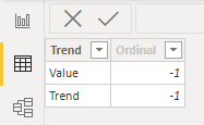
Using Tabular Editor on the sample pbix of my previous post I created a Calculation Group named “Trend Line”, with two Calculation Items: “Value” and “Trend”. Value returns the measure to which it is applied, without any further calculation. Trend instead computes the Linear Regression on the measure.
It’s now possible to create a line chart with the measure and the corresponding trend line by selecting the measure in the Values field and the “Trend Line” calculation group as the Legend
We can now use any measure we please, like for instance the [Margin %]
Now it’s also possible to declare new Trend Line measures without having to copy the full implementation by just applying the existing calculation groups with CALCULATE like
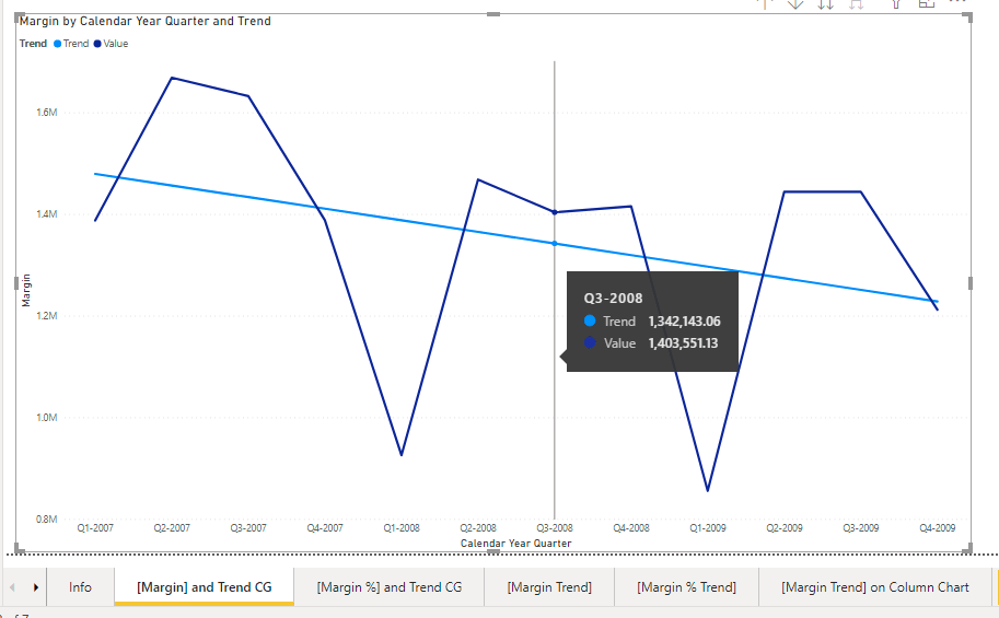
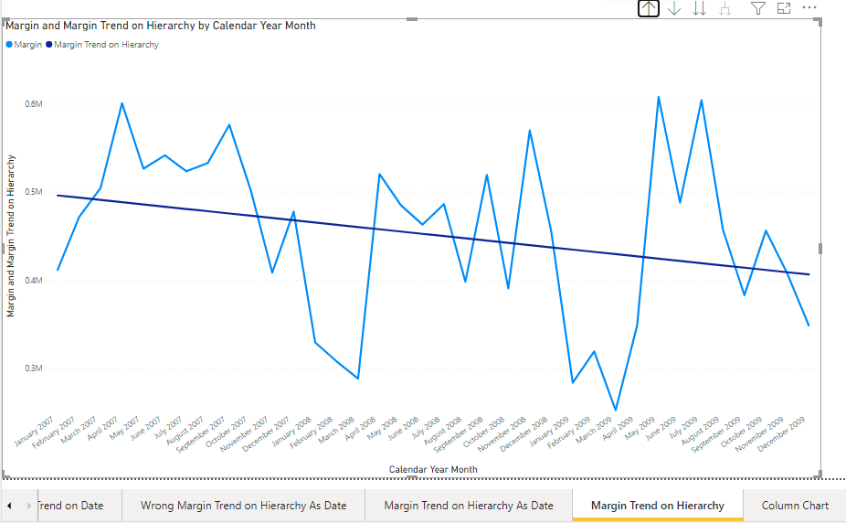
These two measures can be used as the Trend Line measure in the previous post. No calculation group is to be selected for the line chart, but just the [Margin] and the [Margin Trend] measures
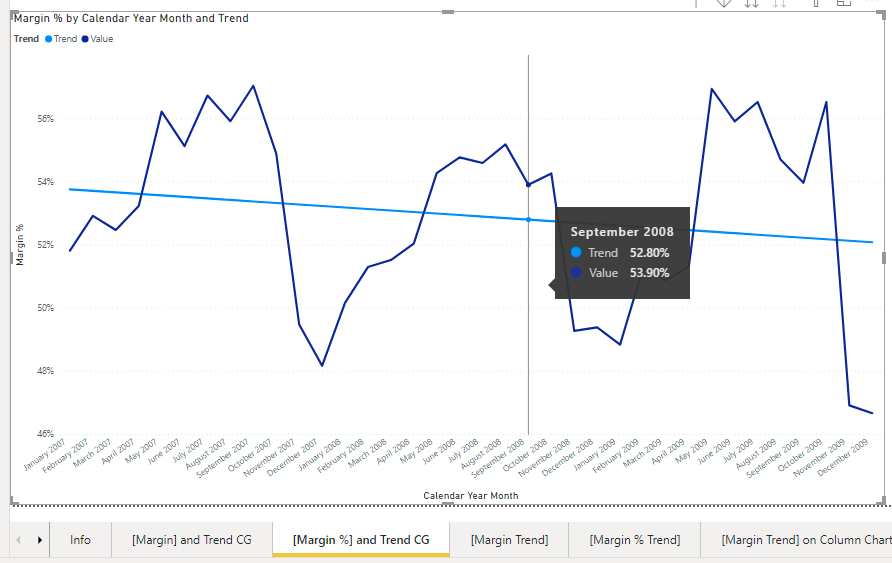
And the same can be done using [Measure %] and [Measure % Trend] measures.
Conclusions
The calculation groups are an effective way to avoid code duplication.
The Trend Line Calculation Group implementation
Calculation Group creation is not supported by the Power BI user interface, but an external tool is required. I used Tabular Editor 2, that is an open source project that can be found on github
As a first step I ran Tabular Editor from the External Tools ribbon in Power BI (I have two versions installed)
Then I selected “Create New -> Calculation Group” from the context menu on “Tables” in the “Model” tree view in Tabular Editor
Then I renamed the column name “Name” to “Trend” and created two new Calculation Items: Value and Trend
Then, using the Expression Editor panel, I implemented the Value calculation item, so that it just returns the current measure using
SELECTEDMEASURE()
And for the Trend calculation item I copy/pasted (one last time) the Linear Regression DAX code for the [Margin] measure and I replaced any reference to the measure [Margin] with SELECTEDMEASURE()
IF (
    NOT ISBLANK ( SELECTEDMEASURE () ),
    SWITCH (
        TRUE,
        ISINSCOPE ( 'Date'[Date] ),
            VAR Tab =
                FILTER (
                    CALCULATETABLE (
                        SELECTCOLUMNS (
                            'Date',
                            "@X", CONVERT ( 'Date'[Date], DOUBLE ),
                            "@Y", CONVERT ( SELECTEDMEASURE (), DOUBLE )
                        ),
                        ALLSELECTED ( 'Date' )
                    ),
                    NOT ISBLANK ( [@X] ) && NOT ISBLANK ( [@Y] )
                )
            VAR SX =
                SUMX ( Tab, [@X] )
            VAR SY =
                SUMX ( Tab, [@Y] )
            VAR SX2 =
                SUMX ( Tab, [@X] * [@X] )
            VAR SXY =
                SUMX ( Tab, [@X] * [@Y] )
            VAR N =
                COUNTROWS ( Tab )
            VAR Denominator = N * SX2 - SX * SX
            VAR Slope =
                DIVIDE ( N * SXY - SX * SY, Denominator )
            VAR Intercept =
                DIVIDE ( SY * SX2 - SX * SXY, Denominator )
            VAR V =
                Intercept
                    + Slope * VALUES ( 'Date'[Date] )
            RETURN
                V,
        ISINSCOPE ( 'Date'[Calendar Year Month] )
            || ISINSCOPE ( 'Date'[Calendar Year Month Number] )
            || ISINSCOPE ( 'Date'[Calendar Year Month As Date] ),
            VAR Tab =
                FILTER (
                    CALCULATETABLE (
                        SELECTCOLUMNS (
                            SUMMARIZE ( 'Date', 'Date'[Calendar Year Month Number] ),
                            "@X", CONVERT ( 'Date'[Calendar Year Month Number], DOUBLE ),
                            "@Y", CONVERT ( SELECTEDMEASURE (), DOUBLE )
                        ),
                        ALLSELECTED ( 'Date' )
                    ),
                    NOT ISBLANK ( [@X] ) && NOT ISBLANK ( [@Y] )
                )
            VAR SX =
                SUMX ( Tab, [@X] )
            VAR SY =
                SUMX ( Tab, [@Y] )
            VAR SX2 =
                SUMX ( Tab, [@X] * [@X] )
            VAR SXY =
                SUMX ( Tab, [@X] * [@Y] )
            VAR N =
                COUNTROWS ( Tab )
            VAR Denominator = N * SX2 - SX * SX
            VAR Slope =
                DIVIDE ( N * SXY - SX * SY, Denominator )
            VAR Intercept =
                DIVIDE ( SY * SX2 - SX * SXY, Denominator )
            VAR V =
                Intercept
                    + Slope * VALUES ( 'Date'[Calendar Year Month Number] )
            RETURN
                V,
        ISINSCOPE ( 'Date'[Calendar Year Quarter] )
            || ISINSCOPE ( 'Date'[Calendar Year Quarter Number] )
            || ISINSCOPE ( 'Date'[Calendar Year Quarter As Date] ),
            VAR Tab =
                FILTER (
                    CALCULATETABLE (
                        SELECTCOLUMNS (
                            SUMMARIZE ( 'Date', 'Date'[Calendar Year Quarter Number] ),
                            "@X", CONVERT ( 'Date'[Calendar Year Quarter Number], DOUBLE ),
                            "@Y", CONVERT ( SELECTEDMEASURE (), DOUBLE )
                        ),
                        ALLSELECTED ( 'Date' )
                    ),
                    NOT ISBLANK ( [@X] ) && NOT ISBLANK ( [@Y] )
                )
            VAR SX =
                SUMX ( Tab, [@X] )
            VAR SY =
                SUMX ( Tab, [@Y] )
            VAR SX2 =
                SUMX ( Tab, [@X] * [@X] )
            VAR SXY =
                SUMX ( Tab, [@X] * [@Y] )
            VAR N =
                COUNTROWS ( Tab )
            VAR Denominator = N * SX2 - SX * SX
            VAR Slope =
                DIVIDE ( N * SXY - SX * SY, Denominator )
            VAR Intercept =
                DIVIDE ( SY * SX2 - SX * SXY, Denominator )
            VAR V =
                Intercept
                    + Slope * VALUES ( 'Date'[Calendar Year Quarter Number] )
            RETURN
                V,
        ISINSCOPE ( 'Date'[Calendar Year] )
            || ISINSCOPE ( 'Date'[Calendar Year Number] )
            || ISINSCOPE ( 'Date'[Calendar Year As Date] ),
            VAR Tab =
                FILTER (
                    CALCULATETABLE (
                        SELECTCOLUMNS (
                            SUMMARIZE ( 'Date', 'Date'[Calendar Year Number] ),
                            "@X", CONVERT ( 'Date'[Calendar Year Number], DOUBLE ),
                            "@Y", CONVERT ( SELECTEDMEASURE (), DOUBLE )
                        ),
                        ALLSELECTED ( 'Date' )
                    ),
                    NOT ISBLANK ( [@X] ) && NOT ISBLANK ( [@Y] )
                )
            VAR SX =
                SUMX ( Tab, [@X] )
            VAR SY =
                SUMX ( Tab, [@Y] )
            VAR SX2 =
                SUMX ( Tab, [@X] * [@X] )
            VAR SXY =
                SUMX ( Tab, [@X] * [@Y] )
            VAR N =
                COUNTROWS ( Tab )
            VAR Denominator = N * SX2 - SX * SX
            VAR Slope =
                DIVIDE ( N * SXY - SX * SY, Denominator )
            VAR Intercept =
                DIVIDE ( SY * SX2 - SX * SXY, Denominator )
            VAR V =
                Intercept
                    + Slope * VALUES ( 'Date'[Calendar Year Number] )
            RETURN
                V
    )
)
Finally I saved the modifications to the model using the Save button
And confirmed the refresh request in the Power BI user inhterface.
Even if Power BI does not support the creation of calculation groups, it fully supports them when they exist in the model, therefore the newly created Trend Line calculation group is now visible in the fields panel as a normal table with a column named “Trend” whose values are “Value” and “Trend”, as can be seen in the Data view panel
An awesome series of articles on Calculation Groups can be found o SQLBI‘s site
The Analytics panel of a few visuals in Power BI provides the Trend Line, that is automatically calculated using the current selection for the visual.
The Trend line panel is available only when the X axis is of numeric type and set to Contiguous, otherwise it is hidden. This is a problem when hierarchies have different types on different levels. For instance on a Date Hierarchy where the Year, the Quarter and the Month are strings obtained through FORMAT and only the Date level is of numeric type.
When the X axis contains a hierarchy, and the the Date level is selected, it’s possible to activate the Trend line from the Analytics panel. But changing the level in the line chart to Year Month, the trend line disappears, and a new “i” icon appears with a tooltip stating that there are “Not a Number” values.
A possible solution is to create a Date Hierarchy where every level is of numeric type and the values are contiguous without “jumps”. For instance, representing the Year Month as YYYYMM, like 200801, 200802 would not work, since after 200812 comes 200901, missing all the values between 200813 and 200899.
An awesome solution is proposed by the SQLBI article Creating a simpler and chart-friendly Date table in Power BI. The idea is to represent each level with a date and then to format the date according to the level. This way, the Year Month value is the date of the end of the month, formatted as “mmmm yyyy”, The Year is the date of the end of the year, formatted as “yyyy” and the Year Quarter is the date of the end of the quarter, formatted as … wait there is no format specifier for the quarter!
This is the graph at the Year Month level
This is the same graph at the Year Quarter level. The format is the same as for the Year Month: “mmmm yyyy”
This might be acceptable, but when a better format for the axis is required, it’s possible to write a “Trend” measure to be used instead of the Analytics Trend line.
The DAX formuia for the “Trend” measure is a straightforward implementation of the Simple Linear Regression, but care must be taken when used with a Date Hierarchy, since it is not additive and the formula has to be implemented for each level of the hierarchy. I “took inspiration” from Daniil Maslyuk’s blog post Simple linear regression in DAX, and I implemented the formula from wikipedia.
This is the resulting line chart with the non-numeric Date Hierarchy at the Year Month level
And at the Year Quarter level
Using the same technique it’s possible to implement other “Trend” measures, for instance a “Total trend” measure to implement a Trend line unaffected by slicers.
Another advantage is that trend measures can be used with visuals that don’t have the Analytics panel.
“Trend” measure DAX code must be replicated per each measure that requires a tend line, and therefore it can be tedious. The usual approach not to replicate DAX code is by using calculation groups. I’m planning to give it a try in the near future.
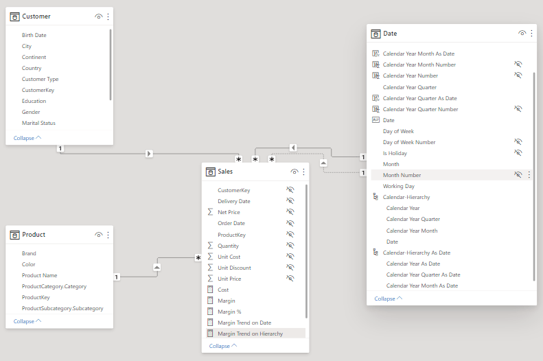
The model
The sample model is built starting from the ContosRetailDW DB that comes with “The Definitive Guide to DAX – Second edition” book companion and is a star schema of the Sales, Customer, Product and Date tables.
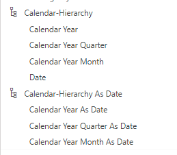
The following calculated columns are needed to build the “Calendar-Hierarchy as Date”, required to implement the solution from the SQLBI article
Calendar Year As Date = ENDOFYEAR( 'Date'[Date] )

Calendar Year Quarter As Date = ENDOFQUARTER( 'Date'[Date] )

Calendar Year Month As Date = ENDOFMONTH( 'Date'[Date] )
The contiguous numeric calculated columns are used for the “Trend” measure
Calendar Year Number = YEAR( 'Date'[Date] ) - YEAR( MIN( 'Date'[Date] ) )

Calendar Year Quarter Number = 'Date'[Calendar Year Number] * 4
    + QUARTER ( 'Date'[Date] ) - 1

Calendar Year Month Number = 'Date'[Calendar Year Number] * 12
    + MONTH( 'Date'[Date] ) - 1
The two “Calendar-Hierarchy” are
The “Trend” measure code
The first version of the “Trend” measure for the [Margin] is the [Margin Trend on Date], that can be used when ‘Date'[Date] is selected for the X axis
Margin Trend on Date =
IF (
    NOT ISBLANK ( [Margin] ),
    VAR Tab =
        FILTER (
            CALCULATETABLE (
                SELECTCOLUMNS (
                    'Date',
                    "@X", CONVERT ( 'Date'[Date], DOUBLE ),
                    "@Y", CONVERT ( [Margin], DOUBLE )
                ),
                ALLSELECTED ( 'Date' )
            ),
            NOT ISBLANK ( [@X] ) && NOT ISBLANK ( [@Y] )
        )
    VAR SX =
        SUMX ( Tab, [@X] )
    VAR SY =
        SUMX ( Tab, [@Y] )
    VAR SX2 =
        SUMX ( Tab, [@X] * [@X] )
    VAR SXY =
        SUMX ( Tab, [@X] * [@Y] )
    VAR N =
        COUNTROWS ( Tab )
    VAR Denominator = N * SX2 - SX * SX
    VAR Slope =
        DIVIDE ( N * SXY - SX * SY, Denominator )
    VAR Intercept =
        DIVIDE ( SY * SX2 - SX * SXY, Denominator )
    VAR V =
        Intercept
            + Slope * VALUES ( 'Date'[Date] )
    RETURN
        V
)
The IF condition is needed to avoid the calculation when the measure for the current date is BLANK().
Then the Tab table variable is declared, to contain all the pairs of Date and Margin values in the filter context of the visual. This is obtained by means of ALLSELECTED( ‘Date’ ) inside CALCULATETABLE(). The conversion to DOUBLE in this sample is needed to avoid an arithmetic overflow caused by multiplications. The remaining code is the straightforward implementation of the Simple Linear Regression formula, to compute the Y for the current ‘Date'[Date].
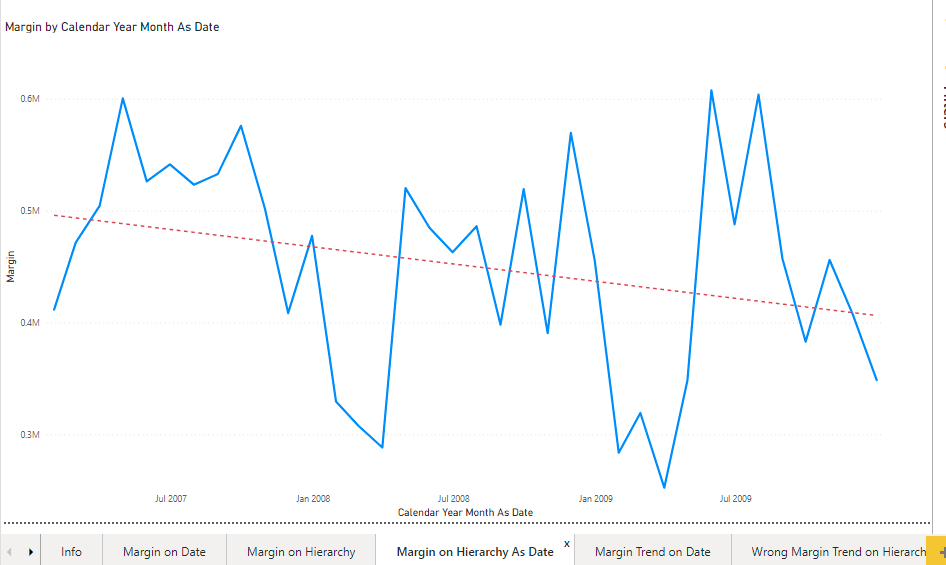
This graph shows the Margin Trend on Date measure perfectly overlapping the Trend line.
But this formula only works when ‘Date'[Date] is set as the X axis. This because the bit of code that computes the V variable makes use of VALUES( ‘Date'[Date] ), that is converted to a scalar value when it contains a single row, but it returns error when it contains more than one row.
VAR V = Intercept + Slope * VALUES ( 'Date'[Date] )
The first idea that comes to mind is to add an aggregator: [Margin] is additive, therefore is [Margin Trend] also additive? The answer is no, because of mathematics.
The following is an attempt (failed attempt) to implement an aggregation that, as expected, does not work
Wrong Margin Trend on Hierarchy =
IF (
    NOT ISBLANK ( [Margin] ),
    VAR Tab =
        FILTER (
            CALCULATETABLE (
                SELECTCOLUMNS (
                    'Date',
                    "@X", CONVERT ( 'Date'[Date], DOUBLE ),
                    "@Y", CONVERT ( [Margin], DOUBLE )
                ),
                ALLSELECTED ( 'Date' )
            ),
            NOT ISBLANK ( [@X] ) && NOT ISBLANK ( [@Y] )
        )
    VAR SX =
        SUMX ( Tab, [@X] )
    VAR SY =
        SUMX ( Tab, [@Y] )
    VAR SX2 =
        SUMX ( Tab, [@X] * [@X] )
    VAR SXY =
        SUMX ( Tab, [@X] * [@Y] )
    VAR N =
        COUNTROWS ( Tab )
    VAR Denominator = N * SX2 - SX * SX
    VAR Slope =
        DIVIDE ( N * SXY - SX * SY, Denominator )
    VAR Intercept =
        DIVIDE ( SY * SX2 - SX * SXY, Denominator )
    VAR V =
        SUMX ( DISTINCT ( 'Date'[Date] ), Intercept + Slope * 'Date'[Date] )
    RETURN
        V
)
And this is the graph showing that the [Wrong Margin Trend on Hierarchy] is not a straight line and even that its own Trend line (purple dotted) doesn’t match with the [Margin] Trend Line (blue dotted)
The correct solution is to test the current hierarchy level with ISINSCOPE and implement the formula accordingly. Which is very long and tedious
Margin Trend on Hierarchy =
IF (
    NOT ISBLANK ( [Margin] ),
    SWITCH (
        TRUE,
        ISINSCOPE ( 'Date'[Date] ),
            VAR Tab =
                FILTER (
                    CALCULATETABLE (
                        SELECTCOLUMNS (
                            'Date',
                            "@X", CONVERT ( 'Date'[Date], DOUBLE ),
                            "@Y", CONVERT ( [Margin], DOUBLE )
                        ),
                        ALLSELECTED ( 'Date' )
                    ),
                    NOT ISBLANK ( [@X] ) && NOT ISBLANK ( [@Y] )
                )
            VAR SX =
                SUMX ( Tab, [@X] )
            VAR SY =
                SUMX ( Tab, [@Y] )
            VAR SX2 =
                SUMX ( Tab, [@X] * [@X] )
            VAR SXY =
                SUMX ( Tab, [@X] * [@Y] )
            VAR N =
                COUNTROWS ( Tab )
            VAR Denominator = N * SX2 - SX * SX
            VAR Slope =
                DIVIDE ( N * SXY - SX * SY, Denominator )
            VAR Intercept =
                DIVIDE ( SY * SX2 - SX * SXY, Denominator )
            VAR V =
                Intercept
                    + Slope * VALUES ( 'Date'[Date] )
            RETURN
                V,
        ISINSCOPE ( 'Date'[Calendar Year Month] )
            || ISINSCOPE ( 'Date'[Calendar Year Month Number] )
            || ISINSCOPE ( 'Date'[Calendar Year Month As Date] ),
            VAR Tab =
                FILTER (
                    CALCULATETABLE (
                        SELECTCOLUMNS (
                            SUMMARIZE ( 'Date', 'Date'[Calendar Year Month Number] ),
                            "@X", CONVERT ( 'Date'[Calendar Year Month Number], DOUBLE ),
                            "@Y", CONVERT ( [Margin], DOUBLE )
                        ),
                        ALLSELECTED ( 'Date' )
                    ),
                    NOT ISBLANK ( [@X] ) && NOT ISBLANK ( [@Y] )
                )
            VAR SX =
                SUMX ( Tab, [@X] )
            VAR SY =
                SUMX ( Tab, [@Y] )
            VAR SX2 =
                SUMX ( Tab, [@X] * [@X] )
            VAR SXY =
                SUMX ( Tab, [@X] * [@Y] )
            VAR N =
                COUNTROWS ( Tab )
            VAR Denominator = N * SX2 - SX * SX
            VAR Slope =
                DIVIDE ( N * SXY - SX * SY, Denominator )
            VAR Intercept =
                DIVIDE ( SY * SX2 - SX * SXY, Denominator )
            VAR V =
                Intercept
                    + Slope * VALUES ( 'Date'[Calendar Year Month Number] )
            RETURN
                V,
        ISINSCOPE ( 'Date'[Calendar Year Quarter] )
            || ISINSCOPE ( 'Date'[Calendar Year Quarter Number] )
            || ISINSCOPE ( 'Date'[Calendar Year Quarter As Date] ),
            VAR Tab =
                FILTER (
                    CALCULATETABLE (
                        SELECTCOLUMNS (
                            SUMMARIZE ( 'Date', 'Date'[Calendar Year Quarter Number] ),
                            "@X", CONVERT('Date'[Calendar Year Quarter Number], DOUBLE),
                            "@Y", CONVERT([Margin], DOUBLE)
                        ),
                        ALLSELECTED ( 'Date' )
                    ),
                    NOT ISBLANK ( [@X] ) && NOT ISBLANK ( [@Y] )
                )
            VAR SX =
                SUMX ( Tab, [@X] )
            VAR SY =
                SUMX ( Tab, [@Y] )
            VAR SX2 =
                SUMX ( Tab, [@X] * [@X] )
            VAR SXY =
                SUMX ( Tab, [@X] * [@Y] )
            VAR N =
                COUNTROWS ( Tab )
            VAR Denominator = N * SX2 - SX * SX
            VAR Slope =
                DIVIDE ( N * SXY - SX * SY, Denominator )
            VAR Intercept =
                DIVIDE ( SY * SX2 - SX * SXY, Denominator )
            VAR V =
                Intercept
                    + Slope * VALUES ( 'Date'[Calendar Year Quarter Number] )
            RETURN
                V,
        ISINSCOPE ( 'Date'[Calendar Year] )
            || ISINSCOPE ( 'Date'[Calendar Year Number] )
            || ISINSCOPE ( 'Date'[Calendar Year As Date] ),
            VAR Tab =
                FILTER (
                    CALCULATETABLE (
                        SELECTCOLUMNS (
                            SUMMARIZE ( 'Date', 'Date'[Calendar Year Number] ),
                            "@X", CONVERT('Date'[Calendar Year Number], DOUBLE),
                            "@Y", CONVERT([Margin], DOUBLE)
                        ),
                        ALLSELECTED ( 'Date' )
                    ),
                    NOT ISBLANK ( [@X] ) && NOT ISBLANK ( [@Y] )
                )
            VAR SX =
                SUMX ( Tab, [@X] )
            VAR SY =
                SUMX ( Tab, [@Y] )
            VAR SX2 =
                SUMX ( Tab, [@X] * [@X] )
            VAR SXY =
                SUMX ( Tab, [@X] * [@Y] )
            VAR N =
                COUNTROWS ( Tab )
            VAR Denominator = N * SX2 - SX * SX
            VAR Slope =
                DIVIDE ( N * SXY - SX * SY, Denominator )
            VAR Intercept =
                DIVIDE ( SY * SX2 - SX * SXY, Denominator )
            VAR V =
                Intercept
                    + Slope * VALUES ( 'Date'[Calendar Year Number] )
            RETURN
                V
    )
)
The ISINSCOPE tests might change according to the existing hierarchies. This sample model has two of them based on different columns.
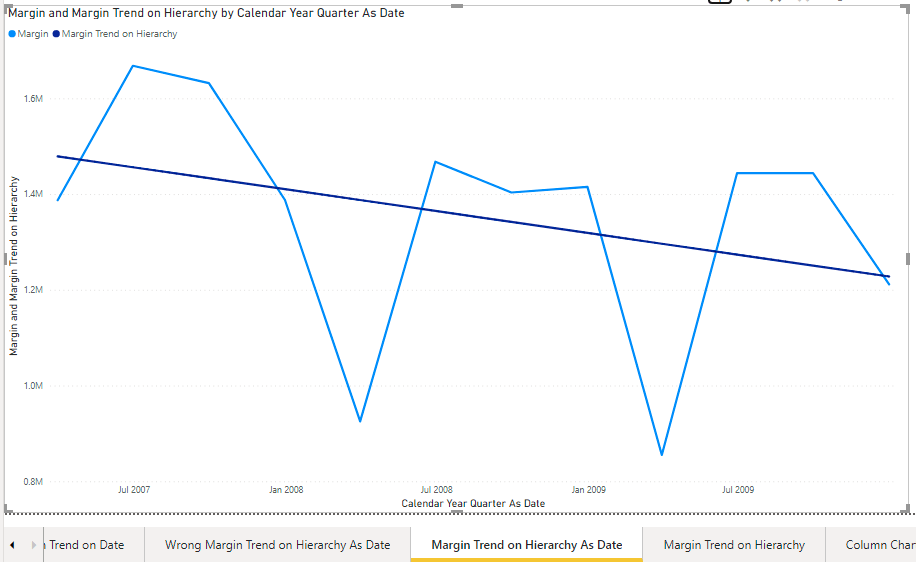
The [Margin Trend on Hierarchy] can be tested against the Trend line using the Calendar-Hierarchy As Date at the Year Month level
And at the Year Quarter level
The Trend line and the [Margin Trend on Hierarchy] overlap just as expected.
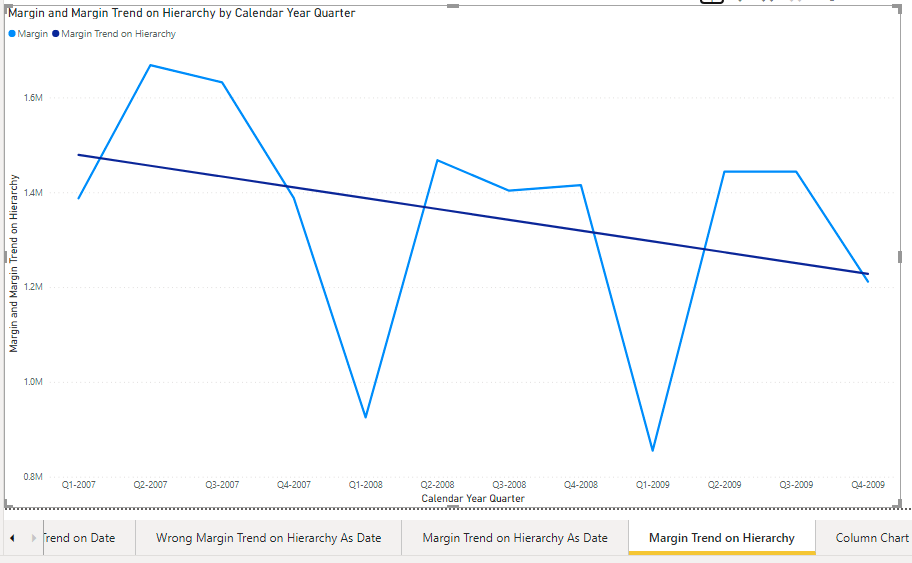
Finally the [Margin Trend on Hierarchy] measure can be used with the plain Calendar-Hierarchy
The [Margin Trend on Hierarchy] can be used with other kind of visuals and even when the [Margin] measure is not selected. Here we have the Margin trend line over a [Sales Amount] per Year Month column chart.
DAX has no duration type, nor a built-in format string to display a duration as days, hours, minutes and seconds.
When the duration is less than one day, an easy solution is to set the column Data Type in the Data View to Time, and then select the Format (hh:nn:ss)
This displays the duration in hours, minutes and seconds as hh:nn:ss (it’s “nn”, since the format “mm” is used for the month)
The problem with longer durations is that when it is more than one day, the days are lost and only the fractional part of the day is shown.
We can see it by entering a duration of 1.5 days, that is shown as 12:00:00, that’s 12 hours instead of 36.
Therefore, in order to display a duration longer than one day, we have to write some DAX code.
The first option is to use the FORMAT function with a custom format string, like for instance “000:00:00:00”. This format string displays a 9 digit number adding the colon as a separator between groups. But writing some code is required in order to build the 9 digit number. The following is a straightforward implementation for a calculated column:
Formatted Duration =
VAR D = T[Duration]
VAR DD = INT(D)
VAR HH = INT(MOD((D * 24), 24))
VAR MM = INT(MOD((D * 24 * 60), 60))
VAR SS = INT(MOD((D * 24 * 60 * 60), 60))
RETURN
FORMAT(DD * 1000000 + HH * 10000 + MM * 100 + SS, "000:00:00:00")
This works, but this code has to be replicated per each column or measure representing a duration.
This is where the calculation groups come into play: if we implement a calculation group to do the formatting, we can write it once and use it in combination with any existing measure.
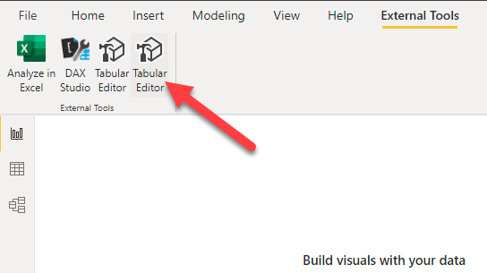
Creating a Calculation Group in Power BI requires Tabular Editor, that can be launched from the External Tools ribbon in Power BI (yes, I have 2 icons of TE in my ribbon: usually only one is installed)
Then using the context menu over the Tables folder we create a new Calculation Group
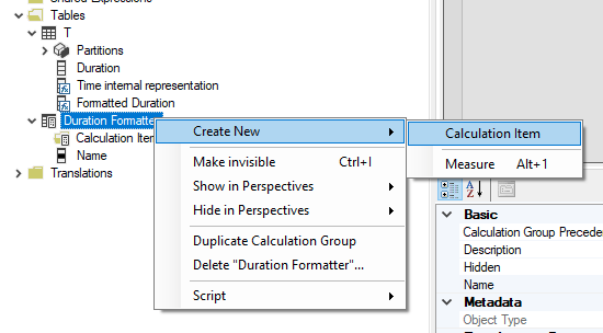
and we give it a meaningful name. I chose “Duration Formatter”
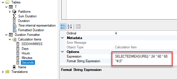
Then using the context menu over the newly created Calculation Group we can create a new Calculation Item
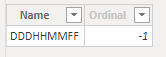
I named it “DDDHHMMSS” and then I wrote the same DAX code as before, just replacing the column reference with the SELECTEDMEASURE() function, and moving the custom format expression to the Format String Expression property
VAR D = SELECTEDMEASURE()
VAR DD = INT(D)
VAR HH = INT(MOD((D * 24), 24))
VAR MM = INT(MOD((D * 24 * 60), 60))
VAR SS = INT(MOD((D * 24 * 60 * 60), 60))
RETURN
DD * 1000000 + HH * 10000 + MM * 100 + SS
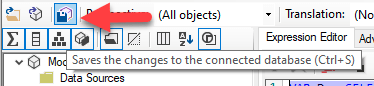
Since Tabular Editor does not synchronize automatically the model to Power BI, we need to save the changes to Power BI by clicking on the Save button in Tabular Editor
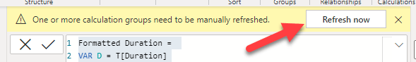
Finally we must click on the Refresh Now button that appears in Power BI
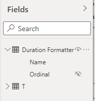
The calculation group can now be seen in Power BI as a table in the data view
To check that the calculation group is working correctly, we can implement a measure
Sum Duration = SUM(T[Duration])
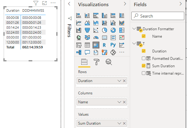
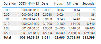
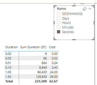
And then use it in a matrix, with the calculation group on the columns
It works! We can now add new Calculation items, to also format the duration as a decimal number representing, for instance, the number of days, or the number of hours, and so on.
Now the matrix with the full CG looks like this
There is a left alignment problem due to the Time data type I set on the Duration column for the first example. But resetting the Duration column data type to “Decimal number” solves the issue.
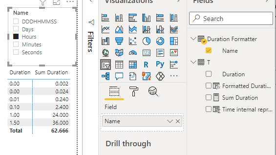
Of course we are not going to use this CG by replicating the same measure with different formats as columns in a matrix. We are most likely going to choose the format to be used with a slicer. So we can remove the CG from the matrix column and create a Slicer instead.
Now we can chose the desired format using the slicer and we can also read the name of the measure instead of the Calculation Item as the column header.
It’s important to know that when selecting two calculation items from the slicer, the CG behaves like when no selection is present.
Wonderful! So everything works fine and we can now use use our Duration Formatter every time a duration requires to be formatted.
No.
Our new toy is now applied to whatever measure happens to be used in our report. For instance, let’s add a measure that calculates a cost, like for instance 1$ per hour
Cost = [Sum Duration] * 24 * 1
When we add this measure to the matrix it gets formatted as if it were a duration.
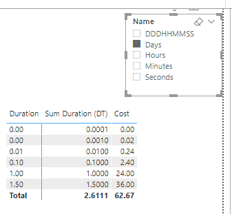
To make the CG only format the duration type measures we must change the code by adding a check on the selected measure name. This can be done by searching a substring that states that the measure represent a duration. For instance we can add the “(DT)” suffix to our measure names and then check for its presence using the SEARCH DAX function.
So I changed the measure definition to
Sum Duration (DT) = SUM(T[Duration])
And the calculation item DDDMMHHSS to
IF (
    SEARCH ( "(DT)", SELECTEDMEASURENAME (), 1, 0 ) > 0,
    VAR D =
        SELECTEDMEASURE ()
    VAR DD =
        INT ( D )
    VAR HH =
        INT ( MOD ( ( D * 24 ), 24 ) )
    VAR MM =
        INT ( MOD ( ( D * 24 * 60 ), 60 ) )
    VAR SS =
        INT ( MOD ( ( D * 24 * 60 * 60 ), 60 ) )
    RETURN
        DD * 1000000 + HH * 10000 + MM * 100 + SS,
    SELECTEDMEASURE()
)
I also added the test to the Format String Expression property as follows
IF (SEARCH("(DT)", SELECTEDMEASURENAME(), 1, 0) > 0, "000:00:00:00")
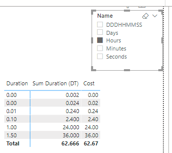
Adding the same test to every calculation item, we are eventually able to use a matrix with both a duration, formatted according to the slicer selection, and a cost, formatted as a decimal number.
Of course a different format string can be used instead of “000:00:00:00”, for instance the format string “000\D\a\y\s 00:00:00” adds the word “Days” after the first three digit group.
In my previous post I implemented the snapshot table for the Events in progress DAX Pattern using DAX. A possible alternative is to build the snapshot table in Power Query using the M language.
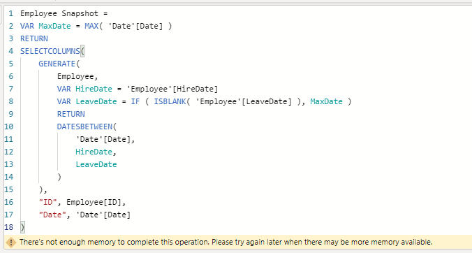
Trying to push further my HR head count model to include the years up to 2015 on my not-so-powerful PC I quickly reached an out of memory error
Therefore I decided to Implement the snapshot table using the M language in Power Query.
This M code is equivalent to the DAX one in my previous post. It takes a few minutes to build the same snapshot table for the 2008-2010 dates interval of the previous post.
let
    LastLeaveDate = #date( 2010, 12, 31 ),
    Source = Employee,
    #"Added Custom" = Table.AddColumn(Source, "Date", each List.Dates(
    [HireDate],
    Duration.Days(
        (
            if [LeaveDate] is null
            then LastLeaveDate
            else [LeaveDate]
        ) - [HireDate]
    ) + 1,
    #duration( 1, 0, 0, 0 )
)),
    #"Expanded Date" = Table.ExpandListColumn(#"Added Custom", "Date"),
    #"Removed Columns" = Table.RemoveColumns(#"Expanded Date",{"Name", "HireDate", "LeaveDate"}),
    #"Changed Type" = Table.TransformColumnTypes(#"Removed Columns",{{"Date", type date}})
in
    #"Changed Type"
I decided to keep it simple, therefore I didn’t implement the code to determine the LastLeaveDate, but I used an inline constant instead.
Then, changing the LastLeaveDate I was able to load the 2008-2015 snapshot table, that failed with the DAX implementation.
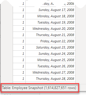
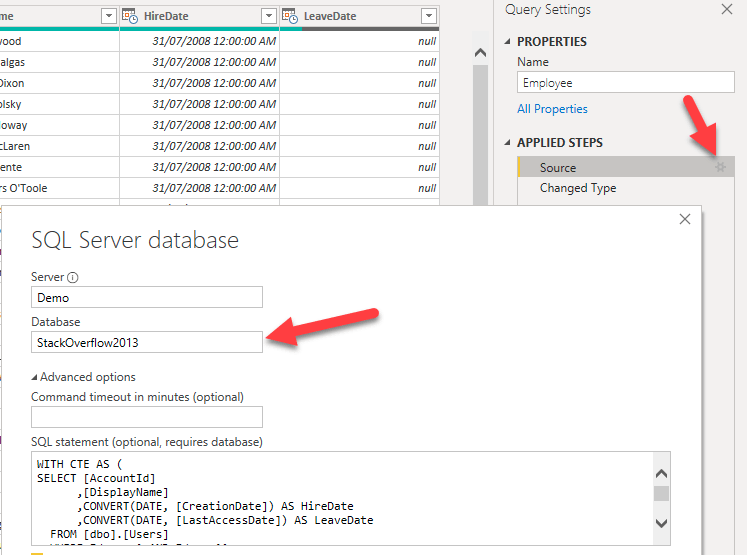
Finally I changed the SQL source DB to StackOverflow2013 (available thanks to Brent Ozar blog), that has a 2.5 Million rows user table. Using this configuration I was able to load a 1.6 Billion rows snapshot table, using my old PC, in about one hour and a half.
The final model size is 2,69 GB and performance of [Head Count Snapshot EOP] measure is still very good.
Implementing the snapshot table using Power Query
As a first step I deleted the Employee Snapshot calculated table in the model and I opened the Transform Data window.
To speed up the refresh time during the development I changed the Source SQL query of the Employee table, to make it load just 100 rows. Clicking on the small gear next to the Source step
I added “TOP 100” to the query after the SELECT
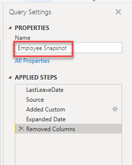
using the context menu over the Employee query in the Queries left panel I added a reference to the Employee query as the first step to the new Employee Snapshot query
Then in the Query settings panel I renamed the new query to Employee Snapshot
At this point we have the same data as the Employee query. We need to add a column containing the list of dates included in the interval between the HireDate and the LeaveDate.
To do so I added a custom column from the Add Column ribbon
Then I added the M code to generate the list of dates, using the M function List.Dates()
List.Dates(start as date, count as number, step as duration) as list
this function takes the start date as first argument, the number of elements of the list to be generated, of type number, and the interval between each two elements, of type duration.
In our scenario the number of elements is the number of days and the step is one day.
The number of elements can be obtained as the difference between the LeaveDate and the HireDate, adding one since both dates must be included. But the difference between two dates returns a duration, therefore I had to use the Duration.Days() function to convert the duration to a number.
The duration can be directly specified using the #duration() function
#duration(days as number, hours as number, minutes as number, seconds as number) as duration
To handle the null LeaveDates I had to use the if then else construct and the #date() function to build the date to be used instead of null
#date(year as number, month as number, day as number) as date
Putting this all together I wrote this custom column formula
= List.Dates(
    [HireDate],
    Duration.Days(
        (
            if [LeaveDate] is null
            then #date( 2010, 12, 31 )
            else [LeaveDate]
        ) - [HireDate]
    ) + 1,
    #duration( 1, 0, 0, 0 )
)
And named the custom column to be created “Date”
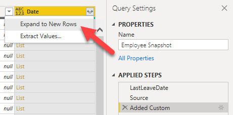
At this point we have a table with the same number of rows as the Employee table, and the same columns plus the new Date columns containing a list. Now we must expand the list in the last column to obtain a table with one row per each day in the list. This can be done using the “Expand to new rows” menu directly on the top of the Date column
Now we can get rid of the Name, HireDate and LeaveDate columns, that are not needed in the snapshot table.
And finally we must convert the type of the Date column from Any to Date
Clicking on Close & Apply, I had to wait a few minutes for the snapshot table generation.
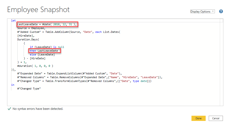
After testing that everything was still working as with the DAX generated snapshot table, I decided to move the #date constant to a variable declared before the step that creates the custom column, so I used the Advanced Editor to open the full M query
and I added the line to declare the LastLeaveDate variable to be used instead of the #date() for the #”Added Custom” step
LastLeaveDate = #date( 2010, 12, 31 ),
The 1.6 Billion Rows model
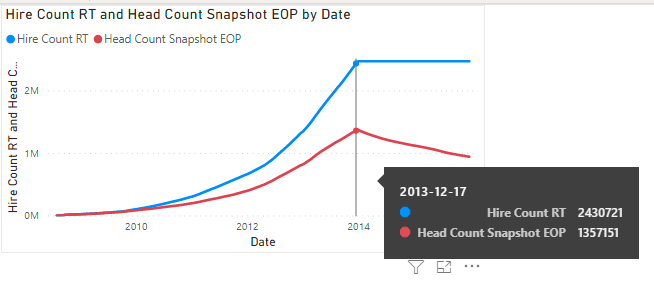
The data used by this big model to simulate the employees are taken from the StackOverflow2013 Users table, that contains the user accounts created on StackOverflow from 2008 to 2013. Therefore the HireDate are simulated from 2008 up to 2013 and LeaveDate from 2008 to 2015.
This means that the head count grows up to the end of 2013 and then just decreases.
The changes from the previous model, the one using StackOverflow2010 DB were just four
First, the Database was changed to StackOverflow2013
Second, the SQL statement in the previous window was changed to force the LeaveDate to NULL after the year 2015
WITH CTE AS (
SELECT [AccountId]
      ,[DisplayName]
      ,CONVERT(DATE, [CreationDate]) AS HireDate
      ,CONVERT(DATE, [LastAccessDate]) AS LeaveDate
  FROM [dbo].[Users]
  WHERE Id <> -1 AND Id <> 11
)
SELECT
	 AccountId AS ID
	,DisplayName AS Name
	,HireDate
	,CASE WHEN LeaveDate > '20151231' THEN NULL ELSE LeaveDate END AS LeaveDate
FROM CTE
Third, the LastLeaveDate in the M code was changed to 2015-12-31
let
    LastLeaveDate = #date( 2015, 12, 31 ),
    Source = Employee,
    #"Added Custom" = Table.AddColumn(Source, "Date", each List.Dates(
    [HireDate],
    Duration.Days(
        (
            if [LeaveDate] is null
            then LastLeaveDate
            else [LeaveDate]
        ) - [HireDate]
    ) + 1,
    #duration( 1, 0, 0, 0 )
)),
    #"Expanded Date" = Table.ExpandListColumn(#"Added Custom", "Date"),
    #"Removed Columns" = Table.RemoveColumns(#"Expanded Date",{"Name", "HireDate", "LeaveDate"}),
    #"Changed Type" = Table.TransformColumnTypes(#"Removed Columns",{{"Date", type date}})
in
    #"Changed Type"
Finally the Date calculated table was expanded to include dates up to the end of 2015
And that’s it. After applying the changes and waited for about 1 hour and a half for the snapshot to be loaded (old PC), I removed the graph using the [Head Count Snapshot ALL] at the day granularity level, that took a long time before failing with an error.
The final pbix takes about 135MB of disk space.
Model Size and Performance
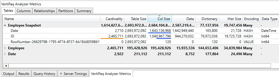
The size of the model as shown by the Vertipaq Analyzer Metrics Summary panel of DAX Studio is 2.69 GB
2.6GB that, as expected, are mainly allocated to the Employee Snapshot table.
To measure performance of the new model I ran the same DAX queries of the previous post using the DAX Studio Server Timings panel.
At first the measure that does not use the snapshot table at the day granularity level, that took 282 seconds
DEFINE
    MEASURE Employee[Head Count] =
        VAR FromDate =
            MIN ( 'Date'[Date] )
        VAR ToDate =
            MAX ( 'Date'[Date] )
        RETURN
            CALCULATE (
                COUNTROWS ( Employee ),
                Employee[HireDate] <= ToDate,
                Employee[LeaveDate] >= FromDate
                    || ISBLANK ( Employee[LeaveDate] ),
                REMOVEFILTERS ( 'Date' )
            )
EVALUATE
SUMMARIZECOLUMNS (
    'Date'[Date],
    "Head_Count", 'Employee'[Head Count]
)
ORDER BY 'Date'[Date]
Then the [Head Count Snapshot ALL] measure, that uses DISTINCTCOUNT on the snapshot table, at the day granularity level. That went rather bad: after several minutes spent swapping memory to the disk it failed with an out of memory error message.
At the day level it’s always possible to use the EOP measure, therefore performance is rather good.
At the month level, when it’s possible to use the EOP measure performance is very good. But if the requirement is to consider the full time interval selection instead of just the last day, then the [Head Count] measure can be used, that at the month level is still acceptable.
The sample pbix file can be downloaded from my GitHub shared project. The big model was too big to be shared, though. Therefore I just shared the pbit.